9 Differential Item Functioning
9.1 Introduction
In Chapter 2, we discussed how testing between-group differences in measurement scores is important for gathering proofs of instrument validity. Similar to testing for the total scores, between-group differences may be inspected on an item level, as was outlined in Chapter 5. However, the proportion of correct answers to an item – the traditional item difficulty estimates – may differ for groups simply because of the differences in their overall ability. In order to analyze the between-group differences in item functioning, the information about item responses, respondent ability, and group membership needs to be combined into a single analysis, often termed a DIF analysis.
The DIF analysis may point to items which are potentially unfair and which need to be evaluated for their content. Analysis of only the between-group differences in total scores or in item scores is not sufficient, as DIF may be present even in cases of identical distribution of the total scores (Figure 9.1, left), and even with significant between-group differences in total scores it is still possible that no item exhibits DIF (Martinková et al., 2017), as illustrated in Figure 9.1 (right).
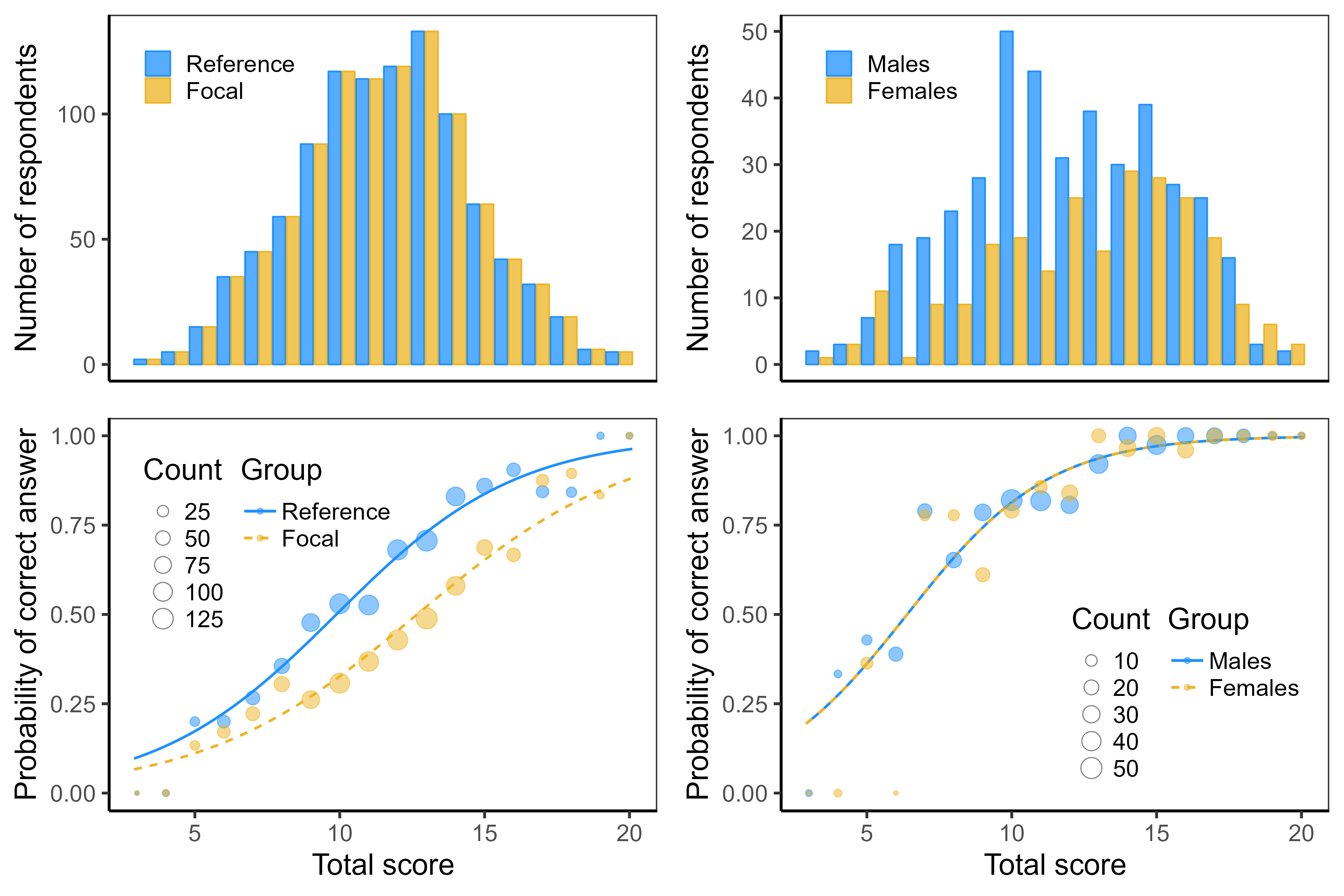
GMAT and HCI. Top: Histograms of total scores. Bottom: Item characteristic curves for selected items. Left: Simulated GMAT dataset with identical observed score distributions (top) but significant DIF in some of the items (bottom). Right: HCI dataset with significant differences in observed scores (top) but no significant DIF item (bottom).
In this chapter, we will introduce several methods for detection of between-group differences in item functioning. In Section 9.3, we will start with the traditional methods which use the ratios of correct answers or mean item scores to test for DIF. These include the Angoff’s Delta plot method (Angoff & Ford, 1973), the MH test (Mantel & Haenszel, 1959), and the SIBTEST (Shealy & Stout, 1993). In Section 9.4, we will look in greater detail into extensions of the regression models from Section 9.4 to account for multiple groups and to test for DIF. In Section 9.5, we will extend the IRT models discussed in Chapter 7 and Chapter 8 to describe and detect DIF. We will mention extensions and combinations of traditional and IRT-based methods in Section 9.6.
9.2 Definition
DIF occurs when respondents with the same underlying true ability, but from different groups, have a different probability of endorsing an item or answering an item correctly. The group membership may be defined by gender, ethnicity, language proficiency, or other categorical variables. When only two groups are compared, they are sometimes denoted as the reference group (e.g., majority) and the focal group (potentially disadvantaged group, e.g., minority). In this chapter, we will focus on detection of DIF in cases involving only two groups; however, the presented concepts may be extended to cases of multiple groups or an even more complex combination of variables defining groups.
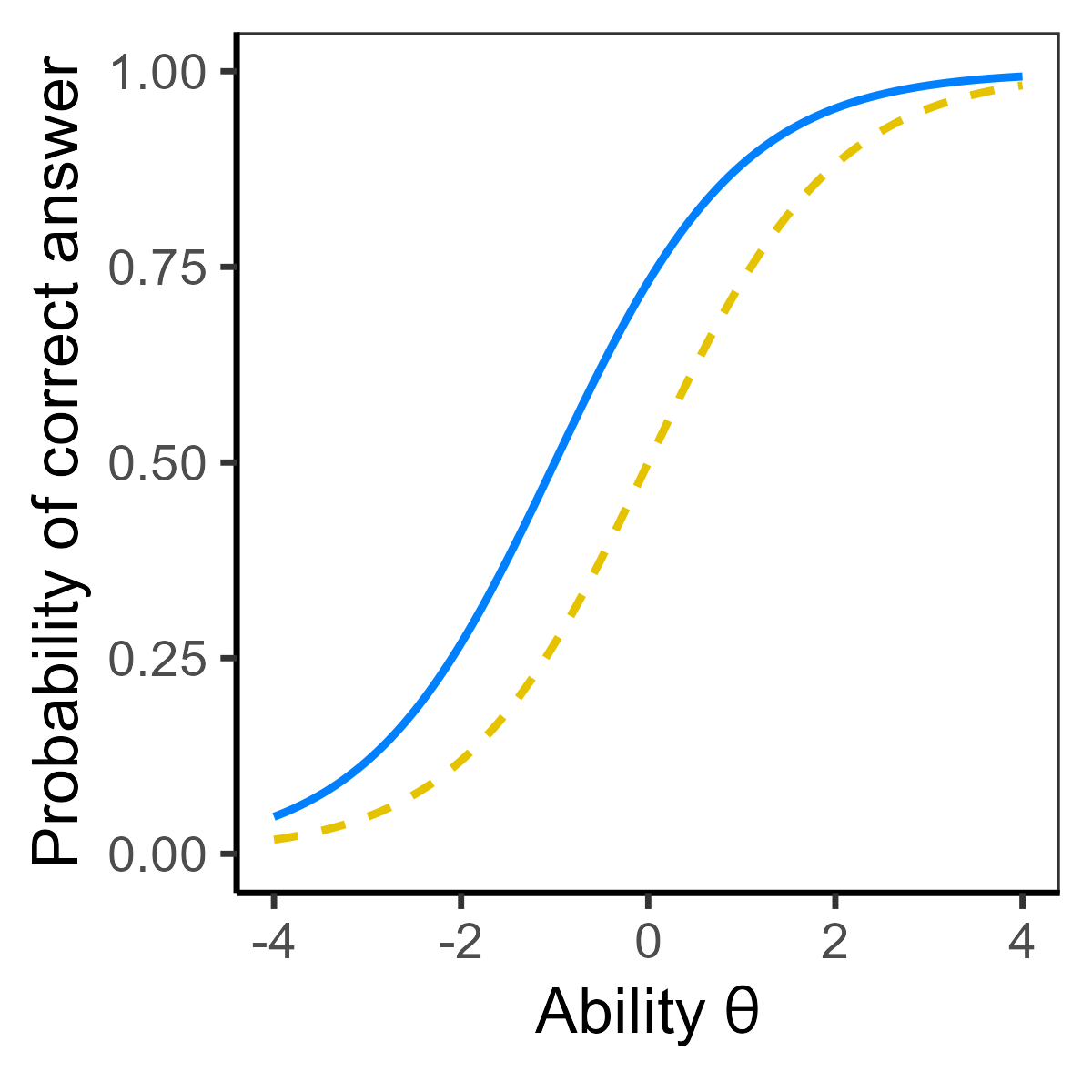
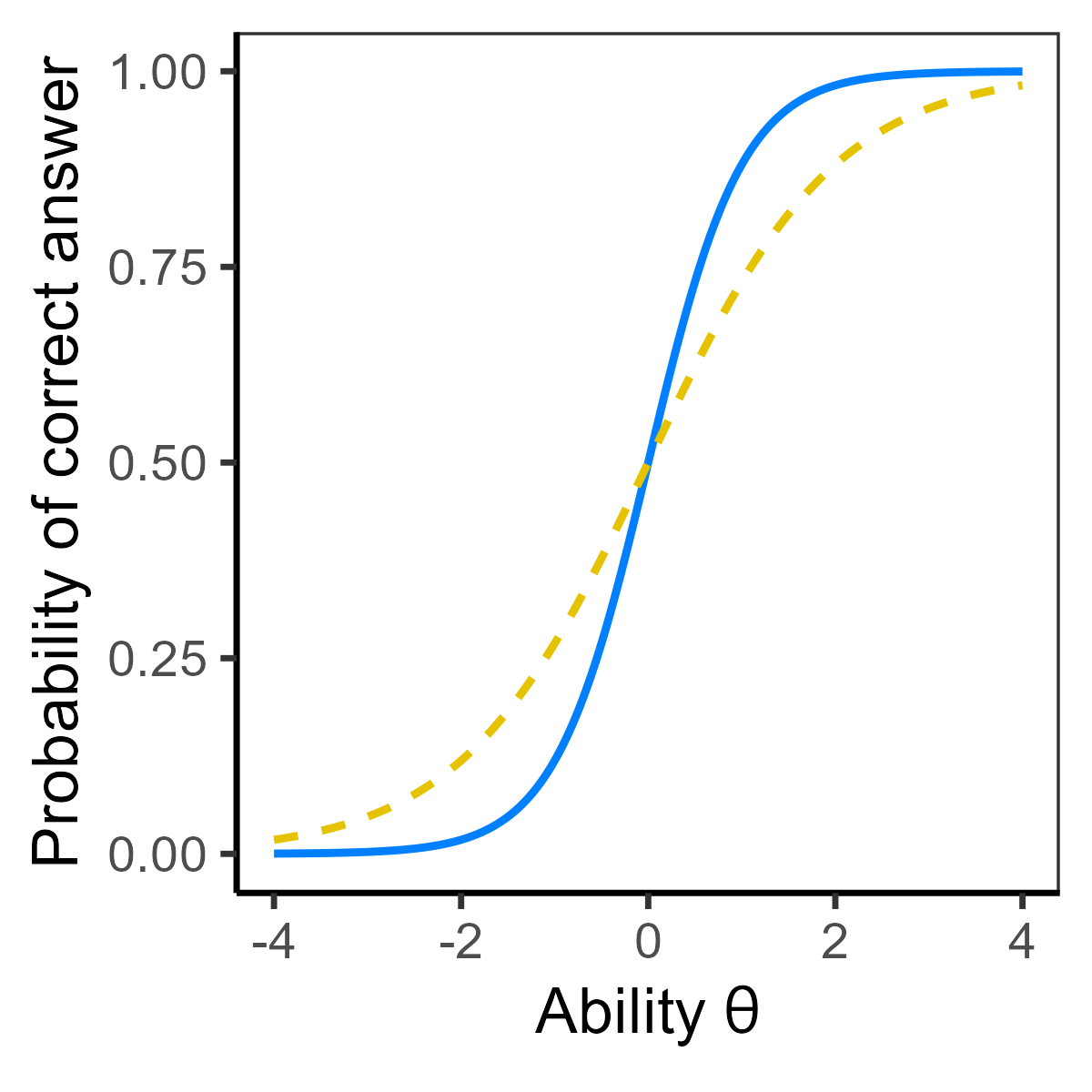
In binary items, we typically distinguish two types of DIF (see, for example, Penfield & Camilli, 2006): In the case of uniform DIF, the item provides a constant relative advantage for the same group across all levels of ability. In this case, the ratio of the odds of answering an item correctly for the focal group compared to the odds for the reference group is a constant (Figure 9.2 (a)). In contrast, in the case of non-uniform DIF, the conditional dependency between an item response and the group membership is not a constant, and it changes across the ability continuum. This may even result in a situation where one group is favored for some levels of ability and the other group is favored for other levels of ability, so-called crossing non-uniform DIF (Figure 9.2 (b)).
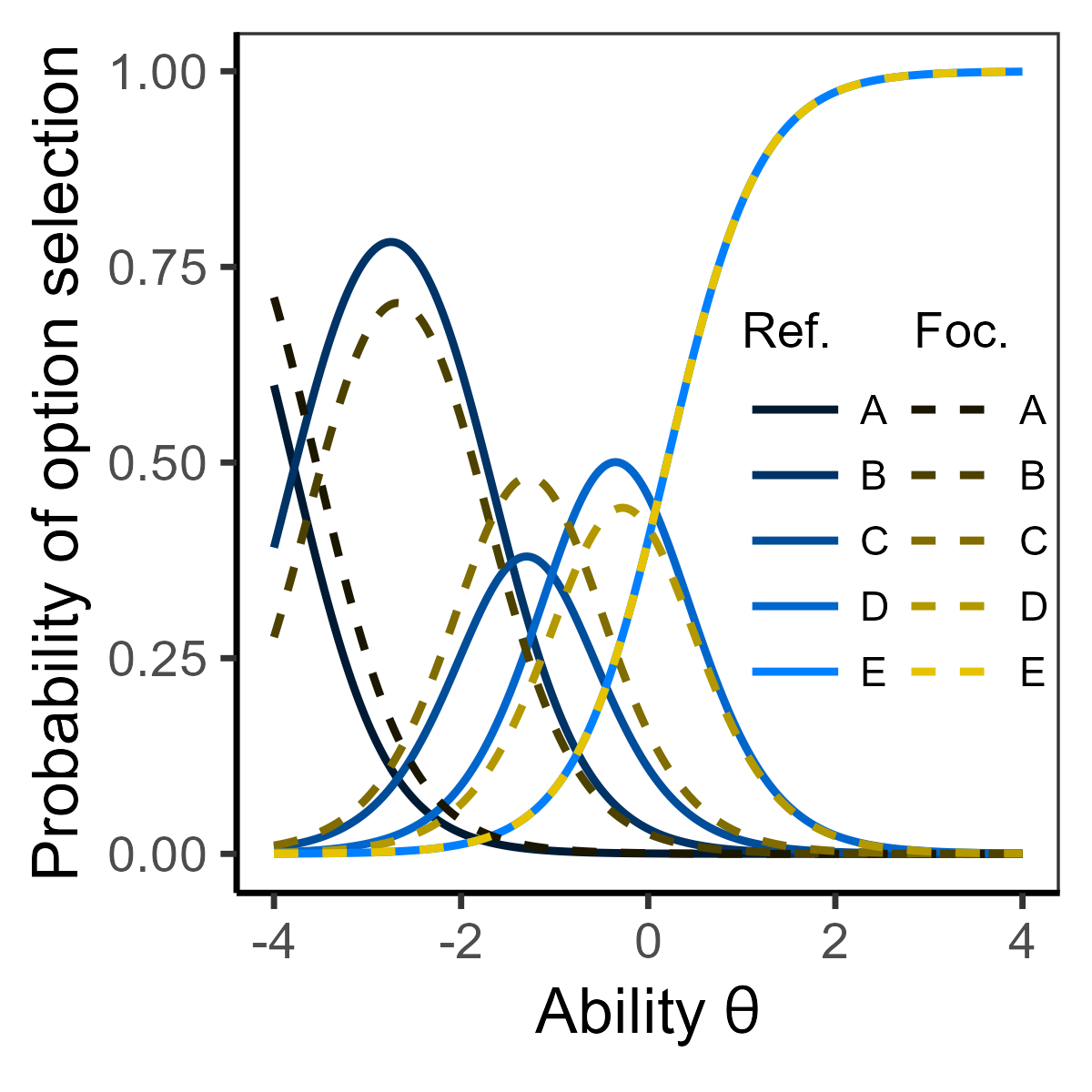
In multiple-choice items, different distractors, i.e., incorrect option choices, may differentially attract respondents with the same ability but from different groups. This phenomenon is termed DDF. In an educational context, DDF analysis is important for detection of misconceptions held by different groups. Note that it may occur that no DIF is detected when a multiple-choice item is scored as a binary item, yet there is DDF detected when the option selection is further analyzed (Figure 9.2 (c)).
9.2.1 DIF examples and interpretations
If an item functions differently for the two groups, it typically means that besides the primary latent trait of interest, the item also measures other (so-called secondary) underlying latent trait(s), and that cognitive differences exist in one of these secondary latent traits (Ackerman, 1992). To decide how such an item should be treated, it is necessary to look closer at the item content and possibly also consider the respondent’s reasoning which can be obtained in so-called “think-aloud interviews”.
If the content experts conclude that the secondary latent trait is irrelevant to the construct being measured, the item is categorized as unfair. This is the case when DIF is caused by unintended item content (such as gender, cultural background, or age of respondents) or some other unintended item property (for example, method of test administration).
A number of DIF items have been reported in the relevant literature. For example, in a questionnaire about pain, the questions “How often did pain prevent you from walking more than 1 mile?” and “How often did pain prevent you from standing for more than 1 hour?” were given a higher grade by older patients than by younger ones with the same overall pain level (Amtmann et al., 2010).
Similarly, in a questionnaire on anger, the older respondents more often endorsed an item on being angry when “people were unfair” or when “they did something stupid” than younger participants with the same level of anger (Pilkonis et al., 2011). In a questionnaire on depression, females tended to endorse more often the statement that they “felt like crying” than males with the same level of depression (Pilkonis et al., 2011).
For many years, the classical example of a DIF item in the context of educational testing was a verbal question involving the word “regatta”, which favored test-takers from wealthier backgrounds, who were also more likely to be white (Cramp & McDougall, 2018). Differences in item responses were concluded to be caused by the fact that a regatta was a typical sport among the white upper class; thus other groups might have been disadvantaged by not understanding the terminology involved. In this case, the item was marked as unfair and removed from the test.
When DIF is detected, however, it does not necessarily mean that the item is unfair. It may be the case that both the primary and secondary latent traits are relevant to the construct being measured. An example of such a case was an item about childhood illnesses from a biology admission test for medical school (Drabinová & Martinková, 2017). DIF analysis revealed that females with the same overall ability performed better than males for this item. Content experts reviewed the item and concluded that the item was fair despite the gender difference, because medical experts need to be familiar with childhood illnesses. In this case, the test writers decided that the secondary latent trait, knowledge of childhood illnesses, was related to the primary concept being tested, which was biology in medicine. Other clear examples of fair items that exhibited DIF exist in literature (Doolittle, 1985; Hamilton, 1999; Liu & Wilson, 2009). Similarly, detected DDF may provide evidence about misconceptions held by different genders or social groups. Even if the item flagged as DIF or DDF is reviewed and concluded to be fair, the act of identifying these gaps in conceptual understanding can influence teaching and, subsequently, help educators and policy makers reduce such gaps in the future.
While most often, the absence of DIF is desirable, in some cases and designs, DIF may be desired. For example, Martinková et al. (2020) used DIF analysis in achievement gains to support the claims of instructional sensitivity, which were not apparent when analyzing only the gains in total scores. Similarly, Kolek et al. (2021) used DIF analysis to further explain effects of a video game on attitude change towards an history event – the expulsion of Sudeten Germans after World War II; in this case the DIF analysis indicated that especially attitudes towards the expulsion’s (un)fairness were affected by the game.
9.2.2 Matching criterion
The choice of the matching criterion also termed matching variable, i.e., the ability estimate by which the respondents from two groups are matched, is crucial for all DIF detection methods. In this chapter we use these terms somewhat interchangeably, all representing an estimate of a latent trait used for DIF analysis.
Traditional methods typically rely upon an observed ability estimate. The natural but not necessary optimal choice might be the total test score or the standardized total score (for discussion see Section Section 6.2). On the other hand, IRT-based methods offer more sophisticated possibilities to estimate a latent trait from item responses. Other options include pretest scores or other related variables to inspect instructional or treatment sensitivity using DIF analysis.
Note that when specifying or estimating the matching variable, DIF items might be present in its calculation, which may be a potential source for bias in DIF detection (see, e.g., Jodoin & Gierl, 2001). Item purification (Candell & Drasgow, 1988; Lord, 1980; Marco, 1977) was proposed to overcome this issue. This algorithm consists of iterative removal of potential DIF items from calculation of the matching criterion which could reduce their possible impact on the matching criterion and, therefore, improve DIF detection (Clauser et al., 1993; French & Maller, 2007), see also Hladká, Martinková, & Magis (2023) for further discussion.
9.3 Traditional DIF detection methods
Various methods have been developed for DIF detection among binary items. Early methods analyzed mainly the mean item scores and proportions of correct answers by the group. These traditional methods are oftentimes easily calculated even by hand. In the sections below, we present three such methods: The Delta plot method, the MH test, and the SIBTEST method.
9.3.1 Delta plot method
Angoff’s Delta plot method (Angoff & Ford, 1973) compares the proportions of correct answers per item between the two groups. The main idea is that under the assumption of invariance of the difficulty parameters (i.e., no DIF), the proportions of correct answers, as difficulty estimates, should lie approximately on a line (which is not necessarily the diagonal).
The Delta plot method takes two extra steps. The first step involves calculating a non-linear transformation of the proportions of correct answers, so-called delta scores. The second step involves calculating the main axis of ellipse which is formed by delta scores. An item is under suspicion of DIF if the delta point deviates considerably from this main axis.
Each DIF detection method has its own strengths as well as its weaknesses. The Delta plot method is easy to compute even without specialized software since it does not require a large sample size, and, moreover, it can account for differences in total score distribution between groups. On the other side, it is only suitable when uniform DIF is present, although it may not be adequate for detection of non-uniform DIF. When item discriminations are not identical for the two groups, some non-DIF items may be incorrectly detected as DIF items, which increases type I error of the method. Additionally, the computation may become problematic when the proportions of correct answers in one of the groups are exactly 0 or 1. In such a case, constraining to a range of [0.05, 0.95] (Angoff & Ford, 1973) or [0.001, 0.999] (Magis & Facon, 2012) should be considered.
To describe the method in more detail, for each item \(i = 1, \dots, m\) and each group (0 – reference and 1 – focal) the proportions of correct answers (the empirical probabilities) are calculated:
\[ \hat{\pi}_{i0} = \frac{1}{n_0}\sum_{p = 1}^{n_0} Y_{pi0} \ \ \text{and} \ \ \hat{\pi}_{i1} = \frac{1}{n_1}\sum_{p = 1}^{n_1} Y_{pi1}, \]
where \(Y_{pi0}\) and \(Y_{pi1}\) are responses on item \(i\) by respondents from the reference and the focal group respectively, and \(n_0\) and \(n_1\) are the number of respondents in the two groups. The standard normal deviates of empirical probabilities are then computed:
\[ z_{i0} = \Phi^{-1}(1 - \hat{\pi}_{i0}) \ \ \text{and} \ \ z_{i1} = \Phi^{-1}(1 - \hat{\pi}_{i1}), \]
where \(\Phi^{-1}\) is a quantile function of the standard normal distribution, i.e., the inverse of the CDF defined in Equation C.4. Finally, the standard normal deviates are transformed into the delta scores:
\[ \Delta_{i0} = 4 z_{i0} + 13 \ \ \text{and} \ \ \Delta_{i1} = 4 z_{i1} + 13. \]
The location of 13 and a slope of 4 are arbitrary and rather historical. Transformed delta scores are on a positive scale, with an average value of 13 and a standard deviation of 4, ranging from 0 to 26 for proportions ranging from 0.001 to 0.999.
Pairs of delta scores \((\Delta_{i0}, \Delta_{i1})\) can be displayed on a scatter plot, also called a delta plot or a diagonal plot, where delta scores of the reference group are on the \(X\) axis and of the focal group on the \(Y\) axis. Delta scores then create an ellipse with a major axis:
\[ \begin{aligned} \Delta_{i1} =& \ a + b \Delta_{i0}, \ \text{where}\\ b =& \ \frac{s_1^2 - s_0^2 + \sqrt{(s_1^2 - s_0^2)^2 + 4s_{01}^2}}{2s_{01}},\\ a =& \ \bar{\Delta}_1 - b \cdot \bar{\Delta}_0, \end{aligned} \]
with \(s_0^2\), \(s_1^2\) being a sample variance of delta scores for the reference and the focal group, \(s_{01}\) their sample covariance, and \(\bar{\Delta}_0\) and \(\bar{\Delta}_1\) their sample means. The formulae for the major axis correspond to the orthogonal least squares regression (Kendall & Stuart, 1967), i.e., the line minimizing orthogonal distances of the points (Figure 9.3). The slope is also identical to the slope of the first component in the principal component analysis (Jackson & Dunlevy, 1988).
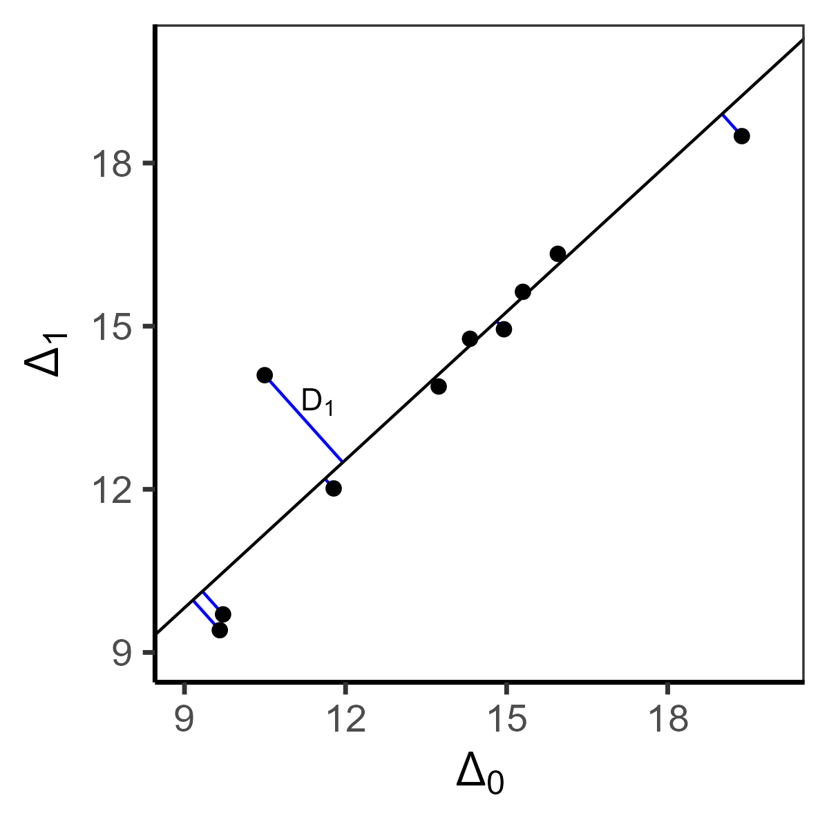
DIF detection is based upon the distance of delta scores from the major axis, which can be calculated as
\[ D_i = \frac{b \Delta_{i0} + a - \Delta_{i1}}{\sqrt{b^2 + 1}}. \]
Calculated distance being large and positive, i.e., a delta point located above the major axis, would suggest that an item is easier for respondents in the reference group. In contrast, a large negative distance, i.e., a delta point below the major axis, would indicate the item was easier for the focal group. In a case where the calculated distance is small, difficulty would be similar for respondents of the same ability from both the reference and focal groups, meaning there would be no DIF in the item.
The crucial point for this method is the selection of a detection threshold to judge whether delta points deviate considerably from the main axis. Typically, a fixed threshold of 1.5 is considered (see, e.g., Muniz et al., 2001). Another option is to use a threshold based upon bivariate normal approximation considering a predefined significance level, which results in distances having standard normal distribution under the null hypothesis (i.e., no DIF) (Magis & Facon, 2012).
Delta plot method in base R. To provide a practical example of implementation, we use the MSATB dataset from the ShinyItemAnalysis package. This dataset contains respondents’ gender (0 – males, 1 – females) and 20 selected scored answers from a medical school admission test in biology (Drabinová & Martinková, 2017), with the first item (item 49) being an item on childhood illnesses functioning differentially with respect to gender already discussed in Section Section 9.2.1. We focus here on the first three items of the dataset, labeled as items \(49\), \(27\), and \(41\).
data(MSATB, package = "difNLR")
head(MSATB, n = 2)
##   Item49 Item27 Item41 ...
## 1      1      0      0 ...
## 2      1      0      1 ...
We must first calculate the empirical probabilities of answering the items correctly for both groups. We use the colMeans() function for this purpose:
(pi0 <- colMeans(MSATB[MSATB$gender == 0, -21]))
## Item49 Item27 Item41 ...
## 0.8161 0.2335 0.3843 ...
(pi1 <- colMeans(MSATB[MSATB$gender == 1, -21]))
## Item49 Item27 Item41 ...
## 0.8776 0.2470 0.3803 ...
The empirical probability of answering item 49 correctly was larger for the female respondents (87.76%) than for males (81.61%). The situation was the opposite in item 41, where male respondents answered correctly more often (38.43%) than females (38.03%); however, the differences in this item were rather negligible.
To calculate the delta scores, we must perform two steps, the calculation of quantiles using the qnorm() function, and their linear transformation.
(z0 <- qnorm(1 - pi0))
##  Item49  Item27  Item41 ...
## -0.9007  0.7275  0.2942 ...
(z1 <- qnorm(1 - pi1))
##  Item49  Item27  Item41 ...
## -1.1629  0.6839  0.3047 ...

(delta0 <- 4 * z0 + 13)
## Item49  Item27  Item41 ...
## 9.3974 15.9099 14.1769 ...
(delta1 <- 4 * z1 + 13)
## Item49  Item27  Item41 ...
## 8.3482 15.7356 14.2190 ...
We should next compute the standard deviations and covariance of the delta scores, and use them to calculate the equation used for the major axis of the ellipse in a form \(y = ax +b\):
s0 <- sd(delta0) # SD of delta scores - males
s1 <- sd(delta1) # SD of delta scores - females
s01 <- cov(delta0, delta1) # covariance of delta scores
mean_delta0 <- mean(delta0) # mean of delta scores - males
mean_delta1 <- mean(delta1) # mean of delta scores - females

(b <- (s1^2 - s0^2 + sqrt((s1^2 - s0^2)^2 + 4 * s01^2))/(2 * s01))
## [1] 0.9784
(a <- mean_delta1 - b * mean_delta0)
## [1] 0.3787
The resulting delta points lie on an ellipse with the main axis with parameters of \(a = 0.38\) and \(b = 0.98\)
We then need to calculate the distance of each delta point from the major axis of the ellipse.
(D <- (b * delta0 + a - delta1) / (sqrt(b^2 + 1)))
## Item49 Item27 Item41 ...
## 0.8753 0.1493 0.0214 ...
For example, the distance for the delta score of item 49 is 0.88. For the MSATB dataset, all of the delta scores are closer to the major axis than the fixed threshold value of 1.5; therefore, no item is detected as functioning differently using the Delta plot method with the fixed threshold.
Delta plot method in the deltaPlotR package. Implementation of the Delta plot method is provided in the deltaPlotR package, and its deltaPlot() function provides a calculation of empirical proportions, their transformation to delta scores, and computation of distances for all items of the dataset. The deltaPlot() function requires specification of data including a grouping variable via the group argument and coding of the focal group through the focal.name argument. We first specify a fixed threshold of 1.5 using the thr argument.
library(deltaPlotR)
(DP_fixed <- deltaPlot(data = MSATB, group = "gender", focal.name = 1, thr = 1.5))
## ...
##        Prop.Ref Prop.Foc Delta.Ref Delta.Foc   Dist.
## Item1    0.8161   0.8776    9.3974    8.3482  0.8753
## Item2    0.2335   0.2470   15.9099   15.7356  0.1493
## Item3    0.3843   0.3803   14.1769   14.2190  0.0214
## ...
## Code: '***' if item is flagged as DIF
## Parameters of the major axis:
##       a       b
##  0.3787  0.9784
## ...
The output includes proportions and delta score for the two groups, calculated distances, and parameters of the major axis. The results are exactly the same as those in our “by hand” calculations above; i.e., no item is detected as functioning differently.
Moreover, the deltaPlot() function offers the possibility to calculate the threshold using a normal approximation as suggested by Magis & Facon (2012). This can be specified via the argument thr = "norm" which is also the default option:
(DP_norm <- deltaPlot(data = MSATB, group = "gender", focal.name = 1,
                      thr = "norm"))
## ...
##        Prop.Ref Prop.Foc Delta.Ref Delta.Foc   Dist.
## Item1    0.8161   0.8776    9.3974    8.3482  0.8753 ***
## Item2    0.2335   0.2470   15.9099   15.7356  0.1493
## Item3    0.3843   0.3803   14.1769   14.2190  0.0214
## ...
## Code: '***' if item is flagged as DIF
##
## Parameters of the major axis:
##       a       b
##  0.3787  0.9784
##
## Detection threshold: 0.606 (significance level: 5%)
## Items detected as DIF items:
## Item1
## ...
While the proportions of correct answers, the delta scores, and their distances from the main axis are the same, contrary to the previous case, these are now compared to a calculated detection threshold of 0.61. Therefore, the first item (item 49) is detected as functioning differently for males and females.
The deltaPlot() function provides other useful options, such as three different types of an iterative purification process (see Section 9.2.2) available via purify and purType arguments (see Supplementary R code).
The deltaPlotR package also offers a graphical display of the delta scores using the diagPlot() function which also plots the major axis. Additionally, with an argument thr.draw = TRUE, the detection threshold may be displayed.
diagPlot(DP_fixed, thr.draw = TRUE)
diagPlot(DP_norm, thr.draw = TRUE)

MSATB dataset.
All delta scores are within limits when using the fixed threshold (Figure 9.4 (a)), while one delta score (for item 49) is outside the area specified by the threshold based upon a normal approximation (Figure 9.4 (b)).
9.3.2 Mantel-Haenszel test
A different approach for the detection of DIF is provided by the MH test (Holland, 1985; Holland & Thayer, 1988), originally developed in the context of biostatistics by Mantel & Haenszel (1959). The MH test is an extension of the \(\chi^2\) test for contingency tables (see, e.g., Agresti, 2002) since it combines contingency tables which are calculated separately for the different levels of total scores.
Similarly to the Delta plot method, the MH test is easy to calculate and use for DIF detection even without specialized software. One disadvantage of this method is that it is unable to detect non-uniform DIF (Exercise 9.1).
To describe this method in more detail, a contingency table for each level of the total score \(k = 1, \dots, m\), is created (Table 9.1), summarizing the number of respondents with a given total score who answered a given item correctly (reference group = \(n_{i01k}\), focal group = \(n_{i11k}\)) or incorrectly (reference group = \(n_{i00k}\), focal group = \(n_{i10k}\)). The item performs similarly for respondents in the reference and focal groups with a given total score of \(k\), if the ratio of the odds of answering the item correctly are close to 1, i.e., \(\frac{n_{i01k} n_{i10k}}{n_{i00k} n_{i11k}} \approx 1\).
| \(Y_i = 1\) | \(Y_i = 0\) | ||
|---|---|---|---|
| Reference group (0) | \(n_{i01k}\) | \(n_{i00k}\) | \(n_{i0\bullet k} = n_{i01k} + n_{i00k}\) |
| Focal group (1) | \(n_{i11k}\) | \(n_{i10k}\) | \(n_{i1\bullet k} = n_{i11k} + n_{i10k}\) |
| \(n_{i\bullet 1k} = n_{i01k} + n_{i11k}\) | \(n_{i\bullet 0k} = n_{i00k} + n_{i10k}\) | \(n_{ik}\) |
To evaluate all levels of the total score simultaneously, MH combines them into a single odds ratio for each item \(i\):
\[ \alpha_{\text{MH}i} = \frac{\sum_{k = 1}^{K} \frac{n_{i01k} n_{i10k}}{n_{ik}}}{\sum_{k = 1}^{K} \frac{n_{i00k} n_{i11k}}{n_{ik}}}, \tag{9.1}\]
where \(n_{ik} = n_{i01k} + n_{i00k} + n_{i11k} + n_{i10k}\) is the number of respondents who gained exactly \(k\) points on the test. The \(\alpha_{\text{MH}i}\) can be seen as a weighted average of odds ratios through all levels of the total score. Values of \(\alpha_{\text{MH}i}\) close to 1 would indicate no DIF. \(\alpha_{\text{MH}i} > 1\) indicates that the reference group is favored in item \(i\), while for the values \(\alpha_{\text{MH}i} < 1\), the focal group has the advantage.
The MH odds ratio \(\alpha_{\text{MH}i}\) Equation 9.1 is often standardized through a log transformation, centering the value around 0 (Zieky, 1993):
\[ \Delta_{\text{MH}i} = -2.35 \cdot \log{(\alpha_{\text{MH}i})}. \tag{9.2}\]
In this case, values of \(\Delta_{\text{MH}}\) close to 0 indicate no DIF. Values less than 0 indicate the reference group being in a favored position while values greater than 0 indicate that the focal group is now in a more favorable position – this change in interpretation being the result of the transformation Equation 9.2.
The values of \(\Delta_{\text{MH}i}\) can be used to determine the DIF effect size (Holland & Thayer, 1985). Category A is linked to a negligible effect and contains items with values of \(|\Delta_{\text{MH}}| < 1\). Category B includes items with a moderate effect determined by values \(1 \leq |\Delta_{\text{MH}}| < 1.5\). Finally, category C incorporates items with a large effect size, i.e., \(|\Delta_{\text{MH}}| \geq 1.5\).
To statistically test for DIF using the MH test, the following test statistic can be used:
\[ \text{MH}_i = \frac{\left[\left|\sum_{k = 0}^{K} \left(n_{i01k} - \frac{n_{i0\bullet k} n_{i\bullet 1k}}{n_{ik}}\right)\right| - 0.5 \right]^2}{\sum_{k = 0}^K \frac{n_{i0\bullet k} n_{i1\bullet k} n_{i\bullet 1k} n_{i\bullet 0k}}{n_{ik}^2 (n_{ik} - 1)}}. \tag{9.3}\]
Note that the terms in the numerator of the \(\text{MH}_i\) statistic Equation 9.3 contain differences between observed and expected numbers for those from the reference group who answered the item correctly, and also incorporates a continuity correction factor of \(-0.5\) (Holland & Thayer, 1988), while the terms in the denominator estimate the variance. Under the null hypothesis of no DIF, the \(\text{MH}_i\) statistic has asymptotically an \(\chi^2\) distribution with 1 degree of freedom (see Section Section C.2.2); values of the \(\text{MH}_i\) are thus compared with a critical value for this distribution (Mantel & Haenszel, 1959).
The Mantel-Haenszel test in base R. To provide a practical example, we will again consider the MSATB dataset and DIF detection with respect to gender. Note that while performed here in R, most of the calculations may easily be done by hand. We start with the calculation in Table 9.1 and with the odds ratio, which is demonstrated for the first item (item 49) and with respondents who have a total score equal to 5 and 12 points. Re-coding of the responses on item 49, which we do with the factor() function, is necessary to preserve ordering in the contingency table.
score <- rowSums(MSATB[, 1:20]) # total score
MSATB$Item49 <- factor(MSATB$Item49, levels = c(1, 0))

# contingency table for item 49 and score 5
(tab1 <- table(MSATB[score == 5, c("gender", "Item49")]))
##       Item49
## gender  1  0
##      0 10  8
##      1 23  9
n_item49_01_5 <- tab1[1, 1]
n_item49_00_5 <- tab1[1, 2]
n_item49_11_5 <- tab1[2, 1]
n_item49_10_5 <- tab1[2, 2]
(n_item49_01_5 * n_item49_10_5) / (n_item49_00_5 * n_item49_11_5)
## [1] 0.4891

# contingency table for item 49 and score 10
(tab2 <- table(MSATB[score == 12, c("gender", "Item49")]))
##       Item49
## gender  1  0
##      0 30  6
##      1 86  8
n_item49_01_12 <- tab2[1, 1]
n_item49_00_12 <- tab2[1, 2]
n_item49_11_12 <- tab2[2, 1]
n_item49_10_12 <- tab2[2, 2]
(n_item49_01_12 * n_item49_10_12) / (n_item49_00_12 * n_item49_11_12)
## [1] 0.9701
For respondents with a total score equal to 5 points, the odds ratio is \(0.49\), suggesting that females (focal group) of this total score have about twice the odds of answering item 49 correctly than the males. For the respondents with a total score of 12 points, the odds ratio is \(0.97\), suggesting the chances for a correct answer are very similar for both males and females at this level of the total score.
Next, the odds ratios for all total score levels are combined by the equation Equation 9.1 into the odds ratio \(\alpha_{\text{MH}i}\) Equation 9.1:
tabs <- xtabs(~ gender + Item49 + score, data = MSATB)

n_item49_01 <- sapply(1:dim(tabs)[3], function(i) tabs[1, 1, i])
n_item49_00 <- sapply(1:dim(tabs)[3], function(i) tabs[1, 2, i])
n_item49_11 <- sapply(1:dim(tabs)[3], function(i) tabs[2, 1, i])
n_item49_10 <- sapply(1:dim(tabs)[3], function(i) tabs[2, 2, i])
n_item49 <- n_item49_01 + n_item49_00 + n_item49_11 + n_item49_10

(alphaMH <- sum(n_item49_01 * n_item49_10 / n_item49) /
    sum(n_item49_00 * n_item49_11 / n_item49))
## [1] 0.5430
The resulting value of the MH odds ratio is \(\alpha_{\text{MH}i} = 0.54\), meaning that, on average, the odds of answering item 49 correctly are about two times lower for males than for females.
We next calculate the standardized odds ratio \(\Delta_{\text{MH}i}\) defined in Equation 9.2.
-2.35 * log(alphaMH)
## [1] 1.4352
The value of the standardized odds ratio \(\Delta_{\text{MH}i}\) is 1.44, which is in line with the conclusions based upon \(\alpha_{\text{MH}i}\), i.e., females being in a favored position for item 49. The value is larger than a borderline value of 1 for category A but lower than 1.5 for category C, defining the moderate (category B) DIF effect size in item 49.
We conclude the calculations by providing the MH statistic Equation 9.3 and the significance test based upon the \(\chi^2\) distribution (see Section Section C.2.2).
n_item49_R <- n_item49_01 + n_item49_00 # reference group
n_item49_F <- n_item49_11 + n_item49_10 # focal group
n_item49_1 <- n_item49_01 + n_item49_11 # correct answers
n_item49_0 <- n_item49_00 + n_item49_10 # incorrect answers

(MHstat <- (abs(sum(n_item49_01 - n_item49_R * n_item49_1 / n_item49)) - 0.5)^2 /
    sum((n_item49_R * n_item49_F * n_item49_1 * n_item49_0) /
          (n_item49^2 * (n_item49 - 1))))
## [1] 12.4456
qchisq(p = 0.95, df = 1)
## [1] 3.8415
(pvalue <- 1 - pchisq(MHstat, df = 1))
## [1] 0.0004

MSATB$Item49 <- as.numeric(paste(MSATB$Item49))
The MH statistic Equation 9.3 for item 49 has a value of 12.45, which is (when using a significance level of 0.05) larger than the critical value of the \(\chi^2\) distribution with 1 degree of freedom at 3.84 (p-value < 0.01). Item 49 is thusly identified as a DIF item. The last line of the code re-codes the responses back to numeric values.
The Mantel-Haenszel test in the difR package. The MH test is implemented in the difR package via its function difMH(). This function expects a data.frame including binary item responses and a binary/factor group identifier. The label for the focal group is provided with the argument focal.name. The output of this function summarizes MH statistics, corresponding p-values, values of \(\alpha_{\text{MH}i}\) and \(\Delta_{\text{MH}i}\), and the classification of DIF effect sizes defined in Equation 9.1–Equation 9.3 and as calculated “by hand” above for all items. We again use the MSATB dataset:
library(difR)
difMH(Data = MSATB, group = "gender", focal.name = 1)
## ...
##          Stat.  P-value
## Item49 12.4456   0.0004 ***
## Item27  0.9159   0.3386
## ...
## Item68  5.0871   0.0241 *
## ...
## Items detected as DIF items:
## Item49
## Item68
##
## Effect size (ETS Delta scale):
## Effect size code:
## 'A': negligible effect
## 'B': moderate effect
## 'C': large effect
##
##        alphaMH deltaMH
## Item49  0.5430  1.4352 B
## Item27  0.8546  0.3693 A
## ...
## Item68  1.3659 -0.7328 A
## ...
## Effect size codes: 0 'A' 1.0 'B' 1.5 'C'
## (for absolute values of 'deltaMH')
## ...
While using the MH test, besides with item 49 shown above, item 68 is also detected as functioning differently (MH = 5.09, df = 1, p-value = 0.02), this time favoring males (reference group); however the DIF effect size for item 68 is negligible (category A).
The difMH() function offers other useful options including specifying anchor (DIF-free) items via the argument anchor to compute the matching criterion, the item purification iterative process via the argument purify, and p-value adjustment for multiple comparisons via an argument p.adjust.method to overcome a possible issue of gradual testing item by item (see Supplementary R code).
9.3.3 SIBTEST
The SIBTEST method (Shealy & Stout, 1993) is based upon between-group differences in the ratios of correct answers for groups defined by total scores. Its modified version, the Crossing-SIBTEST (Chalmers, 2018; Li & Stout, 1996) focuses on detection of non-uniform DIF.
Let \(Y_i\) be the score of item \(i\) and let \(X^{(i)}\) represent the composite score computed as the sum of all items except the currently studied one, i.e,
\[ X^{(i)} = \sum_{j \neq i, j = 1}^m Y_j. \]
The method starts with a calculation for the proportions \(\hat{\pi}_{k}\) (i.e., empirical probabilities) on all respondents who gained a composite score \(X^{(i)} = k\), where \(k\) can take values of \(0, \dots, m - 1\). These proportions are then used as weights for the differences in the mean item scores \(\bar{Y}_{i0k}\) and \(\bar{Y}_{i1k}\) between the respondents with a composite score \(X^{(i)} = k\) from the reference and the focal group, respectively
\[ \hat{\beta}_{i} = \sum_{k = 0}^{m - 1}\hat{\pi}_{k} \left(\bar{Y}_{i0k} - \bar{Y}_{i1k}\right), \tag{9.4}\]
see also Figure 9.5.
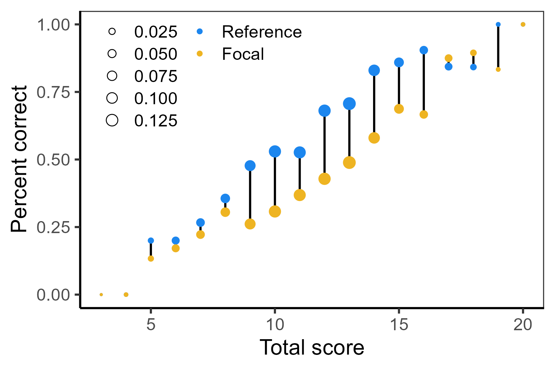
In their paper, illustrating a case for the target ability distributions being the same for both of the groups, Shealy & Stout (1993) derived a formula for \(\hat{\sigma}(\hat{\beta}_i)\), the estimated standard error for the estimate \(\hat{\beta}_i\), and they then proposed a test statistic to identify DIF in item \(i\) in the following form
\[ B_i = \frac{\hat{\beta}_{i}}{\hat{\sigma}(\hat{\beta}_{i})}. \]
Under the null hypothesis of no DIF in item \(i\), i.e., for a case when the true value of \(\beta_{i} = 0\), the test statistic \(B_i\) can be shown to have an asymptotic standard normal distribution.
As in most cases, the assumption of equal ability distributions across groups is an unrealistic condition; therefore, Shealy & Stout (1993) suggested the mean item scores \(\bar{Y}_{i0k}\) and \(\bar{Y}_{i1k}\) in Equation 9.4 be replaced by their regression-based estimates \(\bar{Y}^*_{i0k}\) and \(\bar{Y}^*_{i1k}\), which use a first-order Taylor series of item scores \(\bar{Y}_{i0k}\) and \(\bar{Y}_{i1k}\) by regressing their values toward the true score based upon a composite score.
SIBTEST in the difR package. The SIBTEST method is implemented via the difSIBTEST() function from the difR package. It assumes inputs similar to other functions in this package. Here we show its implementation using the MSATB dataset and DIF detection with respect to gender. The difSIBTEST() function summarizes \(\beta_i\) using regression-based estimates, their standard errors, and corresponding test statistics with p-values.
difSIBTEST(Data = MSATB, group = "gender", focal.name = 1)
## ...
##           Beta      SE X2 Stat. P-value
## Item49 -0.0871  0.0231 14.1465   0.0002 ***
## ...
## Item38 -0.0321  0.0266  1.4620   0.2266
## ...
## Item76  0.0429  0.0276  2.4072   0.1208
## ...
## Detection threshold: 3.841 (significance level: 0.05)
## Items detected as DIF items:
##   Item49
Item 49 is flagged as functioning differently between females and males (\(\chi^2\) = 14.15, df = 1, p-value < 0.01).
To test for non-uniform DIF (Chalmers, 2018) with the difSIBTEST() function, the argument type = "nudif" can be used.
difSIBTEST(Data = MSATB, group = "gender", focal.name = 1, type = "nudif")
## ...
##           Beta    SE X2 Stat. P-value
## Item49  0.0871    NA 14.1465   0.0002 ***
## ...
## Item38  0.0591    NA  7.2962   0.0260 *
## ...
## Item76  0.0593    NA  6.0066   0.0496 *
## ...
## Detection threshold: 3.841 (significance level: 0.05)
## ...
## Items detected as DIF items:
##   Item49
##   Item38
##   Item76
In this case, items 38 and 76 were also detected as DIF items (\(\chi^2\) = 7.30 and 6.01, df = 1, p-values = 0.03 and 0.05 respectively).
Note that the difSIBTEST() function is a wrapper for the SIBTEST() function of the mirt package which we will describe next. The advantages in the implementation of the difR package contain further possibilities including the item purification algorithm or the correction for multiple comparisons (see Supplementary R code).
SIBTEST in the mirt package. In the mirt package, the SIBTEST can be applied with the SIBTEST() function. To test for DIF item by item as we did with the difSIBTEST() function, in the code below, we use the argument suspect_set = i, and we use the function lapply() to apply the function over all items \(i = 1, \dots, m\).
library(mirt)
lapply(1:20, function(i)
    SIBTEST(dat = MSATB[, 1:20], group = MSATB$gender, suspect_set = i))
## [[1]]
##                     focal_group n_matched_set n_suspect_set  beta
## SIBTEST                       0            19             1 0.087
## CSIBTEST                      0            19             1 0.087
##                        SE     X2 df     p
## SIBTEST             0.023 14.146  1 0.000
## CSIBTEST               NA 14.146  1 0.000
## ...
In the output above, we present only the results for the first item (item 49) which correspond to the values obtained from the difSIBTEST() function presented earlier.
9.4 DIF detection based on regression models
Regression models for the description of item functioning described in Section 9.4 can be easily extended to detect DIF by introducing the group membership and its interaction with the respondent’s ability into a model formula. Typically, the standardized total score is used as the matching variable.
9.4.1 Logistic regression
The logistic regression method for DIF detection (Swaminathan & Rogers, 1990) is derived from the logistic model Equation 6.4 for description of item functioning. It extends the model to account for group differences by introducing the effect of the group membership and its interaction with ability. DIF is analyzed by testing for the significance of these terms, in other words, by testing a submodel in which one of these effects (or both) are set at zero.
In the group-specific model, the probability of the correct answer on item \(i\) by respondent \(p\) is given with the following equation:
\[ \Pr(Y_{pi} = 1|X_p, G_p) = \frac{\exp(\beta_{i0} + \beta_{i1} X_{p} + \beta_{i2} G_{p} + \beta_{i3} X_{p}G_{p})}{1 + \exp(\beta_{i0} + \beta_{i1} X_{p} + \beta_{i2} G_{p} + \beta_{i3} X_{p}G_{p})}, \tag{9.5}\]
where \(X_p\) is the ability matching criterion of respondent \(p\), and \(G_p\) is an indicator whether they belong to the focal group (\(G_p = 1\)) or to the reference group (\(G_p = 0\)).
Item parameters are interpreted as follows: Parameter \(\beta_{i0}\) is the model intercept. It gives log-odds for answering item \(i\) correctly by a respondent from the reference group with the ability \(X_p\) of zero:
\[ \beta_{i0} = \log\left(\frac{\Pr(Y_{pi} = 1|X_p = 0, G_p = 0)}{\Pr(Y_{pi} = 0|X_p = 0, G_p = 0)}\right). \]
Note that when the standardized test score is used as the ability matching criterion, the zero value corresponds to the average total test score.
The parameter \(\beta_{i0}\) is therefore linked to the baseline probability of a correct answer with a zero ability for the reference group:
\[ \Pr(Y_{pi} = 1|X_p = 0, G_p = 0) = \frac{\exp(\beta_{i0})}{1 +\exp(\beta_{i0})}. \]
Parameter \(\beta_{i1}\) describes the effect of an ability. It estimates the log-odds ratio for answering item \(i\) correctly when comparing two respondents from the reference group who differ by one point in their observed ability:
\[ \beta_{i1} = \log\left(\frac{\frac{\Pr(Y_{pi} = 1|X_p = x + 1, G_p = 0)}{\Pr(Y_{pi} = 0|X_p = x + 1, G_p = 0)}}{\frac{\Pr(Y_{pi} = 1|X_p = x, G_p = 0)}{\Pr(Y_{pi} = 0|X_p = x, G_p = 0)}}\right). \]
In other words, parameter \(\beta_{i1}\) indicates how the probability of a correct answer on item \(i\) for respondents from the reference group changes (how many times does the log-odds of a correct answer decrease or increase) with an increase of one point in ability.
Parameter \(\beta_{i2}\) is the effect of the group membership. It estimates the log-odds ratio for answering item \(i\) correctly comparing two respondents from the reference group and the focal group with a zero ability:
\[ \beta_{i2} = \log\left(\frac{\frac{\Pr(Y_{pi} = 1|X_p = 0, G_p = 1)}{\Pr(Y_{pi} = 0|X_p = 0, G_p = 1)}}{\frac{\Pr(Y_{pi} = 1|X_p = 0, G_p = 0)}{\Pr(Y_{pi} = 0|X_p = 0, G_p = 0)}}\right). \]
Specifically, parameter \(\beta_{i2}\) determines how the baseline probability of answering item \(i\) correctly differs between the focal group and the reference group. A value of \(\beta_{i2}\) which is significantly larger than zero indicates an advantage for the focal group, while a value significantly lower than zero indicates an advantage for the reference group on a given item. The term \(\beta_{i0} + \beta_{i2}\) is then an intercept for the focal group.
Finally, parameter \(\beta_{i3}\) is the effect of interaction between the ability matching variable and the group membership variable. It describes how the slope is different (a change in the probability of a correct answer on item \(i\) with a one point increase in ability) between the reference group and the focal group. The term \(\beta_{i1} + \beta_{i3}\) is then the effect of ability (the item slope) for the focal group.
IRT parametrization. To estimate group-specific difficulties and discriminations of item \(i\), IRT parametrization of the model Equation 9.5 is often used:
\[ \Pr(Y_{pi} = 1|X_p, G_p) = \frac{\exp((a_i + a_{\text{DIF}i} G_p)(X_p - b_i - b_{\text{DIF}i} G_p))}{1 + \exp((a_i + a_{\text{DIF}i} G_p)(X_p - b_i - b_{\text{DIF}i} G_p))}. \tag{9.6}\]
The variable \(X_p\) is once again the ability matching variable, e.g., a standardized total score. Parameter \(a_i\) can then be interpreted as a discrimination (slope at inflection point) of item \(i\) for the reference group and term \(a_i + a_{\text{DIF}i}\) as a discrimination (slope) for the focal group. Furthermore, parameter \(b_i\) can be seen as a difficulty for item \(i\) of the reference group and term \(b_i + b_{\text{DIF}i}\) as a difficulty for the focal group.
The relationship between item parameters in the classical intercept-slope notation Equation 9.5 and the IRT parametrization Equation 9.6 is as follows:
\[ \begin{alignedat}{3} \beta_{i0} &= -a_i b_i, \quad &&\beta_{i1} = a_i, \\ \beta_{i2} &= -a_i b_{\text{DIF}i} - a_{\text{DIF}i} b_i - a_{\text{DIF}i} b_{\text{DIF}i}, \quad &&\beta_{i3} = a_{\text{DIF}i}, \end{alignedat} \tag{9.7}\]
see Exercise 9.2.
Estimation of parameters. Estimation of the parameters in model Equation 9.5 is typically performed using the ML method and the iterative re-weighted least squares algorithm which was discussed in Section Section 6.5. The relationship Equation 9.7 is used to calculate estimates using the IRT parametrization Equation 9.6, while standard errors for the estimates can be obtained using the delta method Equation 6.10.
9.4.1.1 Testing for DIF
The theoretical values, \(\beta_{i3} = 0\) and \(\beta_{i2} \neq 0\) would correspond to a uniform DIF, while \(\beta_{i3} \neq 0\) would indicate a non-uniform DIF. Testing for DIF itself is, in practice, performed using a test for a submodel. In other words, two competing nested models are to be compared. Here we show two examples of such a test of submodel – the LRT and Wald test.
Likelihood-ratio test. The LRT Equation 2.29 is based upon the idea of assessing the goodness of fit for two competing models, one being a constrained version of the other, and using the ratio of their likelihoods given the observed data. If the constrained model is supported, the difference between the two likelihoods should be small; i.e., their ratio should be close to 1; in other words, the difference of the log-likelihoods should be close to 0. Under the submodel (null hypothesis), the corresponding LRT statistic has an asymptotic \(\chi^2\) distribution Equation C.5 with degrees of freedom equal to the difference in a number of estimated parameters between the model and the submodel (see Sections Section 2.4.2 and Section 2.4.2 for details).
Wald test. Another option is to use the Wald test. The test statistic is given by
\[ W_i = \hat{\boldsymbol{\xi}}_{i, H_\text{alt}}^{\top} \widehat{\mathbb{V}}_{i}^{-1} \hat{\boldsymbol{\xi}}_{i, H_\text{alt}}, \tag{9.8}\]
where \(\hat{\boldsymbol{\xi}}_{i}\) are estimates of item parameters under the larger model (i.e., the model under the alternative hypothesis), and matrix \(\widehat{\mathbb{V}}_{i}\) is an estimate of the corresponding covariance matrix under the larger model \(M_{i}\) restricted to parameters of the submodel. If the null hypothesis holds for item \(i\), then the \(W_i\) statistic has an asymptotic \(\chi^2\) distribution Equation C.5 with degrees of freedom equal to the difference in a number of estimated parameters.
Effect sizes. DIF effect sizes in the logistic regression method are usually categorized based upon Nagelkerke’s \(R^2\) (Nagelkerke, 1991), ranging from 0 to 1. In the categorization by Zumbo & Thomas (1997), the values above 0 (A), above 0.13 (B), and above 0.26 (C), are categorized as negligible (A), moderate (B), or large (C) DIF, respectively. In the categorization by Jodoin & Gierl (2001), the cut values of 0, 0.035, and 0.07, are used instead of the previous values.
To describe the calculation of the effect sizes in more detail, we first define the deviance of the model,
\[ \text{dev}_i = 2 \left[l_i(\hat{\boldsymbol{\xi}}_{i, \text{sat}}) - l_i(\hat{\boldsymbol{\xi}}_{i})\right], \]
as twice the difference in the log-likelihood \(l_i\) Equation 6.14 for the \(\hat{\boldsymbol{\xi}}_{i, \text{sat}}\) parameters estimated under the saturated model, i.e., a model with a parameter for each observation so that the data are fitted exactly, and for the \(\hat{\boldsymbol{\xi}}_{i}\) parameters estimated using the current model. In other words, deviance measures deviation of the model from a model that is a perfect fit to the data. Deviance of a model when only the intercept is considered as a regressor is called null deviance \(\text{dev}_{i, \text{null}}\).
The Nagelkerke’s \(R^2\) for item \(i\) is then defined as
\[ R_i^2 =\ 1 - \left[\exp\left(-\frac{\text{dev}_{i, \text{null}}}{2} + \frac{\text{dev}_{i}}{2}\right)\right]^{2/n}, \]
which is further compared to the Nagelkerke’s \(R^2\) for item \(i\) of the maximal model:
\[ \begin{aligned} R_{i, \text{max}}^2 =&\ 1 - \left[\exp\left(-\frac{\text{dev}_{i, \text{null}}}{2}\right)\right]^{2/n}, \\ R_{i, \text{DIF}}^2 =&\ \frac{R_i^2}{R_{i, \text{max}}^2}. \end{aligned} \]
Finally, the effect size is calculated as a difference between values \(R_{i, \text{DIF}}^2\) when an alternative \(H_\text{alt}\) or null hypothesis \(H_\text{null}\) holds
\[ \Delta R_i^2 = R_{i, \text{DIF}, H_\text{alt}}^2 - R_{i, \text{DIF}, H_\text{null}}^2. \]
However, the values based upon Nagelkerke’s \(R^2\) might tend to be sensitive to sample sizes.
An alternative measure is to use an area between the two estimated Item Characteristic Curves (ICCs), or its weighted version with ability distribution serving as a weight function. Using an analogy from the IRT models, the values above 0.4, 0.6, and 0.8 (respectively, 0.09, 0.12, and 0.14 for the weighted area), can be used as indications of the negligible, moderate, or large DIF effect size (Drabinová & Martinková, 2017).
Logistic regression method with the glm() function. A logistic regression method is easy to run even with base R functions such as glm() which we demonstrate using the MSATB dataset, once again considering DIF detection with respect to gender. We first use the function scale() to calculate the standardized total test score (the Z-score) as a measure of ability. To fit the group-specific model and to test for DIF, we add the gender variable and the interaction between ability and gender as regressors into the model. We then use the LRT of a submodel Equation 2.29 to compare this model fit_alt to its restricted submodel fit_null, which includes only the ability measured by the Z-score, using the anova() method and argument test = "LRT".
zscore <- as.vector(scale(rowSums(MSATB[, 1:20])))
fit_alt <- glm(Item49 ~ zscore * gender, data = MSATB, family = binomial)
fit_null <- glm(Item49 ~ zscore, data = MSATB, family = binomial)
anova(fit_null, fit_alt, test = "LRT")
## Analysis of Deviance Table
##
## Model 1: Item49 ~ zscore
## Model 2: Item49 ~ zscore * gender
##   Resid. Df  Resid. Dev Df Deviance Pr(>Chi)
## 1      1405      982.09
## 2      1403      967.33  2    14.76 0.0006 ***
## ---
## Signif. codes:  0 '***' 0.001 '**' 0.01 '*' 0.05 '.' 0.1 ' ' 1
The \(\chi^2\) statistic has a value of 14.76, which is (using \(\alpha = 0.05\) significance level) larger than the detection threshold of 5.99 (p-value < 0.01); therefore, we conclude that item 49 is functioning differently for females and males.
Alternatively, one may apply the Wald test of a submodel Equation 9.8, for example, by using the wald.test() function from the aod package. Then a covariance matrix and estimated parameters of the larger model fit_alt need to be provided via arguments Sigma and b, while a vector specifying which coefficients should be jointly tested needs to be specified via the Terms argument.
library(aod)
wald.test(Sigma = vcov(fit_alt), b = coef(fit_alt), Terms = c(3, 4))
## ...
## Chi-squared test:
## X2 = 14.8975, df = 2, P(> X2) = 0.0006
When using the Wald test, item 49 is again flagged as a DIF item (\(W\) = 14.90, df = 2, p-value < 0.01).
The predict() method can be used on the glm object to obtain the estimated probability of a correct answer for a respondent of a given group and matching criterion. We present below an estimation of the probability of a correct answer for respondents from the reference group and the focal group with ability levels of \(-1\), \(0\), and \(1\), specified in the argument newdata, for the larger model fit_alt.
predict(fit_alt, newdata = data.frame(zscore = c(-1, 0, 1),
        gender = 0), type = "response")
##      1      2      3
## 0.6457 0.8660 0.9582
predict(fit_alt, newdata = data.frame(zscore = c(-1, 0, 1),
        gender = 1), type = "response")
##      1      2      3
## 0.7819 0.9215 0.9747
For all three levels of the standardized total score, the probability of a correct answer is larger for respondents from the focal group, suggesting uniform DIF in item 49.
To extract parameters from the glm object with standard errors, one can use the summary() method.
summary(fit_null)
## ...
##              Estimate Std. Error z value Pr(>|z|)
## (Intercept)    2.2231     0.1060   20.97   <2e-16 ***
## zscore         1.1860     0.1026   11.56   <2e-16 ***
## ...
summary(fit_alt)
## ...
##               Estimate Std. Error z value Pr(>|z|)
## (Intercept)     1.8659     0.1582   11.79  < 2e-16 ***
## zscore          1.2659     0.1671    7.58  3.6e-14 ***
## gender          0.5973     0.2147    2.78   0.0054 **
## zscore:gender  -0.0797     0.2142   -0.37   0.7099
## ...
The effect of gender presented by parameter \(\beta_{i2} = 0.60\) (SE = 0.21) and coded as gender in the output above, is positive, indicating a higher baseline probability for female respondents. On the other hand, a negative value for the interaction parameter \(\beta_{i3} = -0.08\) (SE = 0.21), coded as zscore:gender, suggests that with an increasing standardized total test score the probability steeps slightly less for females. However, the effect of interaction is small and not significant, which is in line with our previous belief of uniform DIF in item 49.
The glm() function uses the classical intercept-slope parametrization as in Equation 9.5. The model parameters under the IRT parametrization Equation 9.6 can be obtained from the relationship Equation 9.7. We use the setNames() function to rename elements of the vector.
a <- coef(fit_alt)[2]
b <- -coef(fit_alt)[1] / coef(fit_alt)[2]
aDIF <- coef(fit_alt)[4]
bDIF <- (coef(fit_alt)[1] * coef(fit_alt)[4] - coef(fit_alt)[2] *
    coef(fit_alt)[3]) / (coef(fit_alt)[2] * (coef(fit_alt)[2] + coef(fit_alt)[4]))
setNames(c(a, b, aDIF, bDIF), c("a", "b", "aDIF", "bDIF"))
##      a       b    aDIF    bDIF
## 1.2659 -1.4740 -0.0797 -0.6025
The standard deviations of the new group-specific item parameters can be obtained using the delta method Equation 6.10.
library(msm)
deltamethod(list(~ x2, ~ -x1 / x2, ~ x4, ~ (x1 * x4 - x2 * x3) / (x2 * (x2 + x4))),
            mean = coef(fit_alt), cov = vcov(fit_alt))
## [1] 0.1671 0.1584 0.2142 0.2374
This item is rather easy: A standardized total score of \(-1.47\) (SE = 0.17) is needed to answer the item correctly with 50% probability for males and a somewhat lower standardized total score of \(-1.47 + (- 0.60) = -2.07\) needed for females. The slopes are almost identical, considering the fact that interaction between Z-scores and group variable is non-significant, and about 1.3 in both groups.
Logistic regression method in the difR package. A logistic regression method is implemented in the difR package and its function difLogistic(). The syntax of the function is analogous to the difMH() and difSIBTEST() functions. As a default, this function uses the total score as a measure of observed ability which serves as a matching for the group-specific model. A standardized total score can instead be used with the argument match = "zscore". Other available arguments allow for the implementation of item purification (purify), or for the corrections of multiple comparisons (p.adjust.method); see Supplementary R code.
Output of the difLogistic() function summarizes the likelihood-ratio statistics, the corresponding p-values, and DIF effect sizes based upon Nagelkerke’s \(R^2\).
(fit_LR <- difLogistic(Data = MSATB, group = "gender", focal.name = 1))
## ...
##        Stat.   P-value
## Item49 14.7603  0.0006 ***
## Item27  1.2130  0.5453
## Item41  0.6366  0.7274
## ...
## Items detected as DIF items:
## Item49
##
## Effect size (Nagelkerke's R^2):
## Effect size code:
##  'A': negligible effect
##  'B': moderate effect
##  'C': large effect
##        R^2    ZT JG
## Item49 0.0164 A  A
## Item27 0.0007 A  A
## Item41 0.0003 A  A
## ...
## Effect size codes:
##  Zumbo & Thomas (ZT): 0 'A' 0.13 'B' 0.26 'C' 1
##  Jodoin & Gierl (JG): 0 'A' 0.035 'B' 0.07 'C' 1
## ...
Only item 49 has been detected as functioning differently (\(LR\) = 14.76, df = 2, p-value < 0.01), while its DIF effect size is negligible considering both classifications based on Nagelkerke’s \(R^2\). Note that test statistics and corresponding p-values are the same as with the glm() functions although here we used a total test score instead of standardized scores as the matching variable.
The difLogistic() function also offers the Wald test of a submodel Equation 9.8 via the criterion = "Wald" argument.
difLogistic(Data = MSATB, group = "gender", focal.name = 1, criterion = "Wald")
## ...
##          Stat. P-value
## Item49 14.8975  0.0006 ***
## Item27  1.1941  0.5504
## Item41  0.6420  0.7254
## ...
Results are once more the same as those from the wald.test() function from the aod package.
Parameters given by the best fitted model from the fit_LR (saved output of the difLogistic() function) can be found in the logitPar value as a matrix with rows representing items and columns representing estimated parameters in intercept-slope parametrization Equation 9.5.
fit_LR$logitPar[1, ]
## (Intercept)       SCORE       GROUP SCORE:GROUP
##     -1.7668      0.3281      0.8259     -0.0206
Note that parameters now differ from those estimated with the glm() function above, as the total test score was used as the matching criterion.
The difR package offers a plot of ICCs via the plot() method using the argument plot = "itemCurve" (Figure 9.6 (a)). Alternatively, one can use the plotDIFLogistic() function from the ShinyItemAnalysis package which offers a graphical environment of the ggplot2 package (Figure 9.6 (b)).
library(ShinyItemAnalysis)
plot(fit_LR, plot = "itemCurve")
plotDIFLogistic(fit_LR, item = 1, Data = MSATB[, 1:20], group = MSATB[, 21])
difR package.
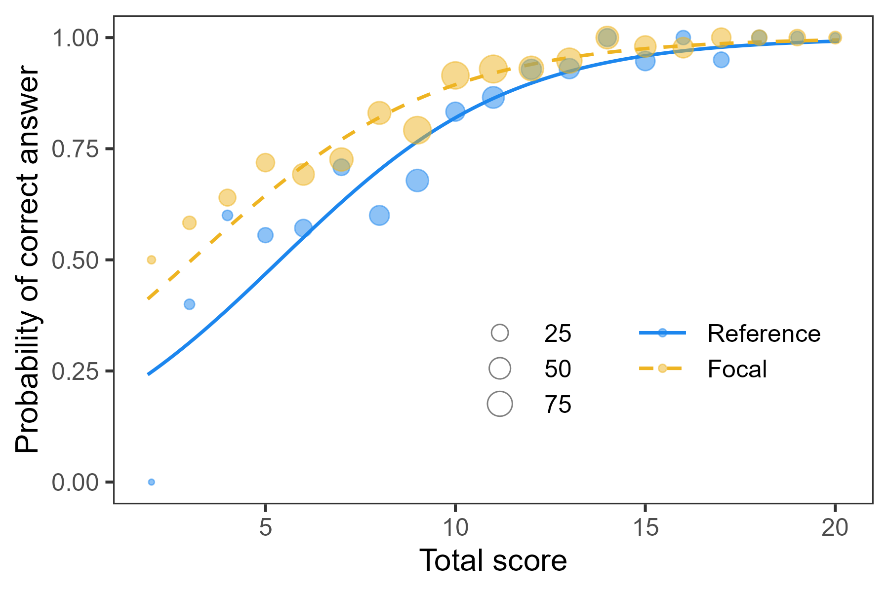
ShinyItemAnalysis package.
MSATB dataset with different packages.
Logistic regression method in the difNLR package. While designed for generalizations of the logistic regression models, which will be described in the next section, the DIF can also be tested under the logistic regression model in the difNLR package with its difNLR() function. This function offers various estimation methods (including nonlinear least squares as the default option and ML with different algorithms) which can be specified via the method argument. Estimation based on ML using an iteratively reweighted least squares algorithm as in the glm() or difLogistic() functions can be applied for the 2PL model with the argument method = "irls". Further, the difNLR() function offers, by default, a standardized total score as the ability matching criterion. The output summarizes test statistics (LRT being the default option) and corresponding p-values. Estimated parameters with 95% confidence intervals can be printed using the coef() method. It is also possible to print them in intercept-slope parametrization Equation 9.5 by specifying IRTpars = FALSE or complement them by standard errors via SE = TRUE or without confidence intervals using CI = 0 (see Supplementary R code).
library(difNLR)
(fit_NLR_2PL <- difNLR(Data = MSATB, group = "gender", focal.name = 1,
                       model = "2PL", method = "irls"))
## ...
##        Chisq-value P-value
## Item49 14.7603      0.0006 ***
## Item27  1.2130      0.5453
## Item41  0.6366      0.7274
## ...
## Items detected as DIF items:
## Item49
coef(fit_NLR_2PL)$Item49
##               a       b    aDif    bDif
## estimate 1.2659 -1.4740 -0.0797 -0.6025
## CI2.5    0.9384 -1.7845 -0.4994 -1.0678
## CI97.5   1.5934 -1.1634  0.3401 -0.1371
Values of test statistics and corresponding p-values are once more the same as those obtained above. Estimated item parameters for item 49 are equal to those estimated by the glm() function using the IRT parametrization Equation 9.6.
The final model can be plotted with the plot() method which uses a graphical environment of the ggplot2 package. Besides ICCs, it also plots the empirical probabilities for both groups and each level of the standardized total score similarly to the plotDIFLogistic() function from the ShinyItemAnalysis package.
plot(fit_NLR_2PL, item = "Item47")In the case of non-DIF item 47, the estimated ICCs are the same for both groups (Figure 9.7 (a)).
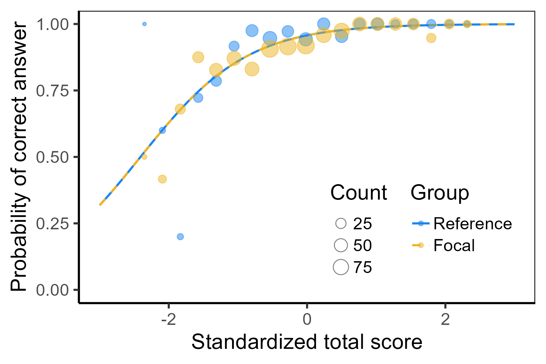
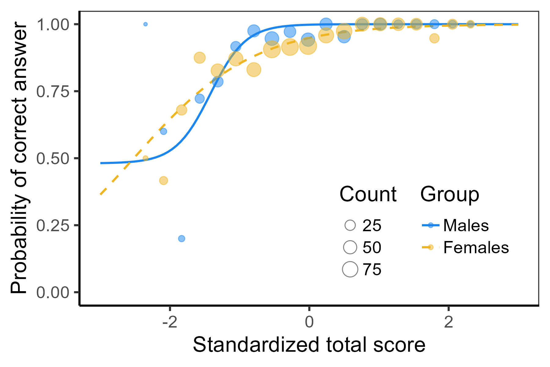
MSATB dataset with the difNLR package.
9.4.2 Generalized logistic regression models
Similarly to a simple logistic regression model Equation 6.4, models Equation 9.5 and Equation 9.6 can also be extended to account for the possibility of guessing or inattention when answering, and to test for between-group differences in these item parameters (Drabinová & Martinková, 2017; Hladká, 2021; Hladká & Martinková, 2020). Using the IRT parametrization with \(X_p\) being the ability matching criterion, e.g., standardized total score, and \(G_p\) the group membership variable, the probability of a correct answer on item \(i\) by respondent \(p\) is then given by
\[ \begin{split} \Pr(Y_{pi} = 1|X_p, G_p) =& \ c_i + c_{\text{DIF}i} G_p + (d_i + d_{\text{DIF}i} G_p - c_i - c_{\text{DIF}i} G_p) \\ & \ \cdot \frac{\exp((a_i + a_{\text{DIF}i} G_p)(X_p - b_i - b_{\text{DIF}i} G_p))}{1 + \exp((a_i + a_{\text{DIF}i} G_p)(X_p - b_i - b_{\text{DIF}i} G_p))}. \end{split} \tag{9.9}\]
The new parameter \(c_i\) corresponds to guessing in item \(i\) in the reference group, i.e., the lower asymptote of the ICC. The parameter \(c_{\text{DIF}i}\) is the difference in guessing between the reference group and the focal group; thus \(c_i + c_{\text{DIF}i}\) is the guessing parameter for the focal group. Similarly, the new parameters \(d_i\), and \(d_i + d_{\text{DIF}i}\) describe respondent inattention in the two groups, i.e., the upper asymptotes of the ICC. Analogously to the 4PL model Equation 6.12, new parameters for reference and the focal group represent probabilities and, therefore, are constrained to an interval \([0, 1]\).
Estimation of parameters and testing for DIF. Estimation of the parameters in model Equation 9.9 is a bit more demanding than in the logistic regression model Equation 9.5. This is due both to the nonlinear nature of the model and to the constraints set on the lower and upper asymptotes. Possible options for estimating item parameters include, for example, the nonlinear least squares (see Section Section 6.5.1) or the ML method (see Section Section 6.5.2); see also Hladká, Martinková, & Brabec (2023) for discussion.
DIF detection offers a number of different models and submodels. These include, as special cases, testing for uniform and non-uniform DIF. Testing for submodels is typically done with the LRT, but an F-test or Wald’s test may also be used (Drabinová & Martinková, 2017; Hladká, 2021).
Generalized logistic model in the difNLR package. The generalized logistic regression method Equation 9.9 is implemented in the difNLR package and its difNLR() function. The syntax is similar to the functions from the difR package. The output summarizes the likelihood-ratio statistics and the corresponding p-values. Below, we present this function using the MSATB dataset and consider DIF detection with respect to gender.
Since the MSATB dataset consists of multiple-choice items, we expect guessing, while no inattention by the respondents is anticipated. Therefore, we use the argument model = "3PLc" to fit the 3PL model for which the inattention parameter \(d_i\) is fixed to a value of 1 and \(d_{\text{DIF}i} = 0\). Estimated parameters and ICCs may again be displayed using the coef() and plot() methods respectively.
(fit_NLR_3PL <- difNLR(Data = MSATB, group = "gender", focal.name = 1,
                       model = "3PLc"))
## ...
##        Chisq-value P-value
## Item49 22.3978      0.0001 ***
## ...
## Item47  9.5320      0.0230 *
## ...
## Items detected as DIF items:
## Item49
## Item47
coef(fit_NLR_3PL)$Item47
##               a       b       c    aDif    bDif    cDif
## estimate 3.9562 -1.4195  0.4807 -2.7970 -1.0999 -0.4807
## CI2.5    1.2439 -1.7505  0.2290 -5.6017 -4.7142 -3.0727
## CI97.5   6.6684 -1.0886  0.7325  0.0077  2.5144  2.1112
plot(fit_NLR_3PL, item = "Item47", group.names = c("Males", "Females"))
Besides item 49, item 47 is now also observed to be functioning differently (\(LR\) = 9.53, df = 3, p-value = 0.02). Estimated parameters for item 47 suggest there is quite a large difference in guessing between male and female respondents (also see Figure 9.7 (b)). While females were estimated not to be guessing at all, males were estimated to be guessing in 48.07% of the cases. However, the corresponding confidence interval is wide.
9.4.3 Group-specific cumulative logit model
To test for DIF among ordinal items, extension of the cumulative logit model Equation 6.18 may be considered, allowing for group-specific item parameters. Using the intercept-slope parametrization and considering \(K_i + 1\) ordered outcome categories for item \(i\), i.e., \(Y_{pi} \in \left\{0, 1, \dots, K_i\right\}\), the probability of gaining at least \(k = 1, \dots, K_i\) points by respondent \(p\) on item \(i\) is
\[ \Pr(Y_{pi} \geq k|X_p, G_p) = \frac{\exp\left(\beta_{i0k} + \beta_{i1} X_p + \beta_{i2} G_p + \beta_{i3} X_pG_p\right)}{1 + \exp\left(\beta_{i0k} + \beta_{i1} X_p + \beta_{i2} G_p + \beta_{i3} X_pG_p\right)}, \tag{9.10}\]
while it equals to 1 for \(k = 0\), i.e., \(\Pr(Y_{pi} \geq 0|X_p, G_p) = 1\).
Interpretation of the parameters is as follows: The \(K_i\) parameters \(\beta_{i0k}\) are the \(k\) category-specific intercepts within item \(i\), ordered by the category index \(k\), i.e., \(\beta_{i01} < \beta_{i02} < \dots < \beta_{i0K_i}\). The parameter \(\beta_{i1}\) is an item-specific slope which is assumed to be the same for all categories \(k\). The parameter \(\beta_{i2}\) describes the effect of group membership. Finally, the parameter \(\beta_{i3}\) defines the difference in slopes, as it is associated with the effect of interaction between the ability matching criterion \(X_p\) and the group membership variable \(G_p\). In total, we end up with \(K_i + 3\) parameters to estimate item \(i\).
The category probability, i.e., the probability of gaining exactly \(k\) points in item \(i\), can be calculated as the difference between the cumulative probabilities of two adjacent categories:
\[ \Pr(Y_{pi} = k|X_p, G_p) = \Pr(Y_{pi} \geq k|X_p, G_p) - \Pr(Y_{pi} \geq k + 1|X_p, G_p), \]
for categories \(k = 0, \dots, K_i - 1\), while for \(k = K_i\) it is
\[ \Pr(Y_{pi} = K_i|X_p, G_p) = \Pr(Y_{pi} \geq K_i|X_p, G_p). \]
Estimation of parameters follows the procedures analogous for the logistic regression model from Section 9.4. Testing for DIF can be performed using the LRT.
IRT parametrization. Analogously to the logistic regression model for DIF detection Equation 9.5, the IRT parametrization can be applied for the cumulative logit model Equation 9.10 to estimate group-specific difficulties and discriminations:
\[ \Pr(Y_{pi} \geq k|X_p, G_p) = \frac{\exp\left((a_{i} + a_{\text{DIF}i}G_p)(X_p - b_{ik} - b_{\text{DIF}ik}G_p)\right)}{1 + \exp\left((a_{i} + a_{\text{DIF}i}G_p)(X_p - b_{ik} - b_{\text{DIF}ik}G_p)\right)}. \tag{9.11}\]
Parameters \(b_{ik}\) describe \(k\) category-specific difficulty for the reference group, i.e., the ability needed for having 50% probability of gaining at least \(k\) points in item \(i\). Parameters \(b_{\text{DIF}ik}\) are then \(k\) category-specific differences in difficulties between the focal group and the reference group. Parameter \(a_i\) represents the slope of cumulative probability curves for the reference group in item \(i\), and it is assumed to be the same for all categories within a given item. Finally, parameters \(a_{\text{DIF}i}\) describe a difference in slope between the focal group and the reference group in item \(i\).
The mutual relationship between parameters using the two parametrizations in models Equation 9.10 and Equation 9.11 is as follows:
\[ \begin{split} a_{i} =&\ \beta_{i1}, \quad \qquad a_{\text{DIF}i} =\ \beta_{i3}, \\ b_{ik} =&\ -\frac{\beta_{i0k}}{\beta_{i1}}, \quad b_{\text{DIF}ik} =\ \frac{\beta_{i0k}\beta_{i3} - \beta_{i1}\beta_{i2}}{\beta_{i1}\left(\beta_{i1} + \beta_{i3}\right)}; \end{split} \tag{9.12}\]
see Exercise 9.3. Standard errors for the parameter estimates in the IRT parametrization Equation 9.11 can be calculated using the delta method Equation 6.10.
Group-specific cumulative logit model in the difNLR package. The cumulative logit model for DIF detection among ordinal items is implemented in the difORD() function of the difNLR package. Here we illustrate its usage by performing DIF detection with respect to gender (0 – males, 1 – females) in the Anxiety dataset using standardized total score as the matching criterion. The output of the function summarizes the LRT statistics and corresponding p-values.
data(Anxiety, package = "ShinyItemAnalysis")
Anxiety_items <- Anxiety[, paste0("R", 1:29)]

(fit_ORD1 <- difORD(Data = Anxiety_items, group = Anxiety$gender, focal.name = 1,
                    model = "cumulative"))
## ...
##     Chisq-value P-value
## ...
## R6  13.8917      0.0010 ***
## R7   9.3795      0.0092 **
## R8   1.2370      0.5388
## ...
## R19  9.0748      0.0107 *
## R20 10.6796      0.0048 **
## R21  5.9576      0.0509 .
## ...
## Items detected as DIF items:
## R6
## R7
## R10
## R19
## R20
Besides others, item R6 “I was concerned about my mental health” was detected to be functioning differently for males and females (\(LR\) = 13.89, df = 2, p-value < 0.01).
Analogously to the difNLR() function, the estimated model parameters can be extracted using the coef() method which offers both the intercept-slope parametrization Equation 9.10 and the IRT parametrization Equation 9.11; Again the choice can be specified via the argument IRTpars – default value TRUE prints estimated coefficients in the IRT parametrization Equation 9.11. Here we do not print standard errors or confidence intervals.
coef(fit_ORD1, SE = FALSE, CI = 0)$R6
##     b1     b2     b3     b4      a
## 0.2248 1.1264 2.1714 3.2289 2.1390
##  bDIF1  bDIF2  bDIF3  bDIF4   aDIF
## 0.3112 0.2811 0.2462 0.2109 0.0738
The cumulative and category response functions for the final model can be displayed using the plot() method (Figure 9.8).
plot(fit_ORD1, item = "R6", plot.type = "cumulative",
     group.names = c("Males", "Females"))
plot(fit_ORD1, item = "R6", plot.type = "category",
     group.names = c("Males", "Females"))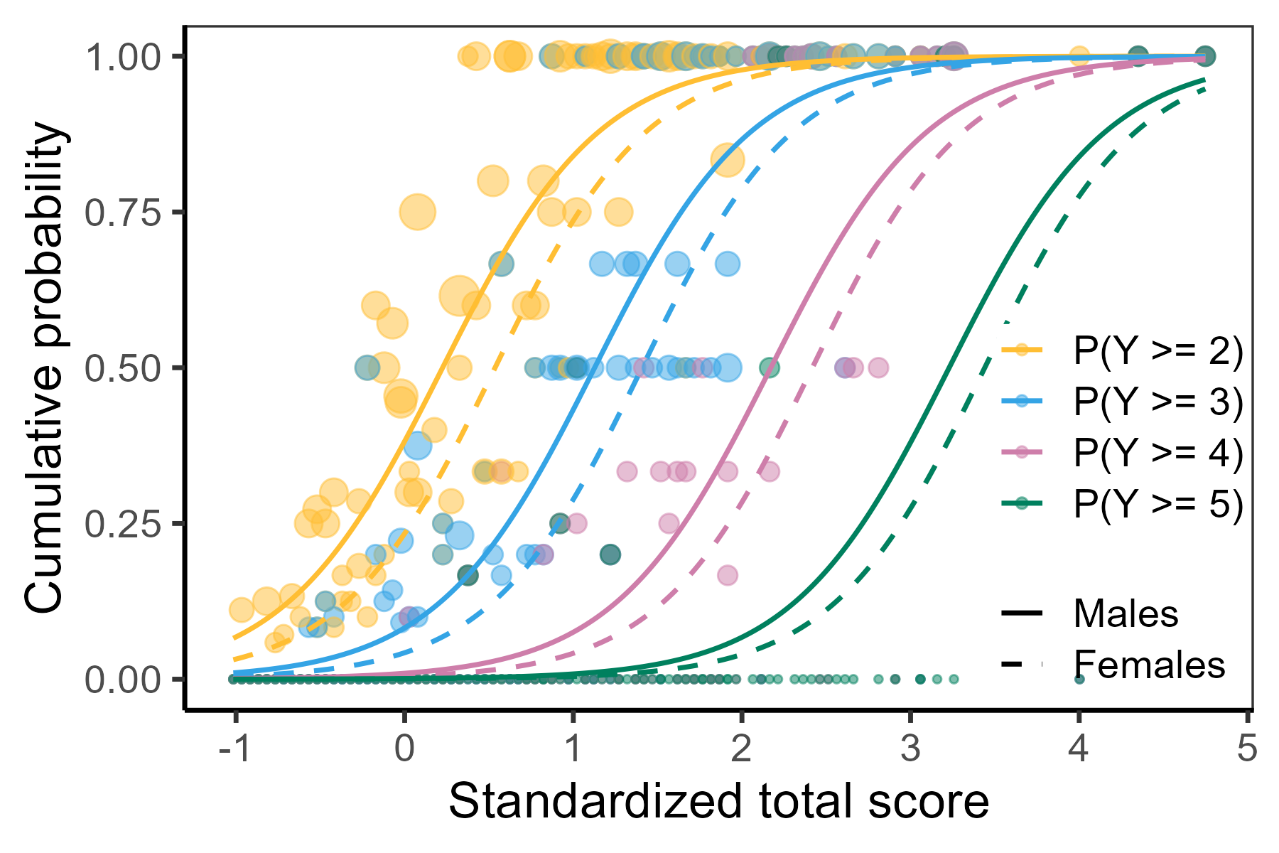
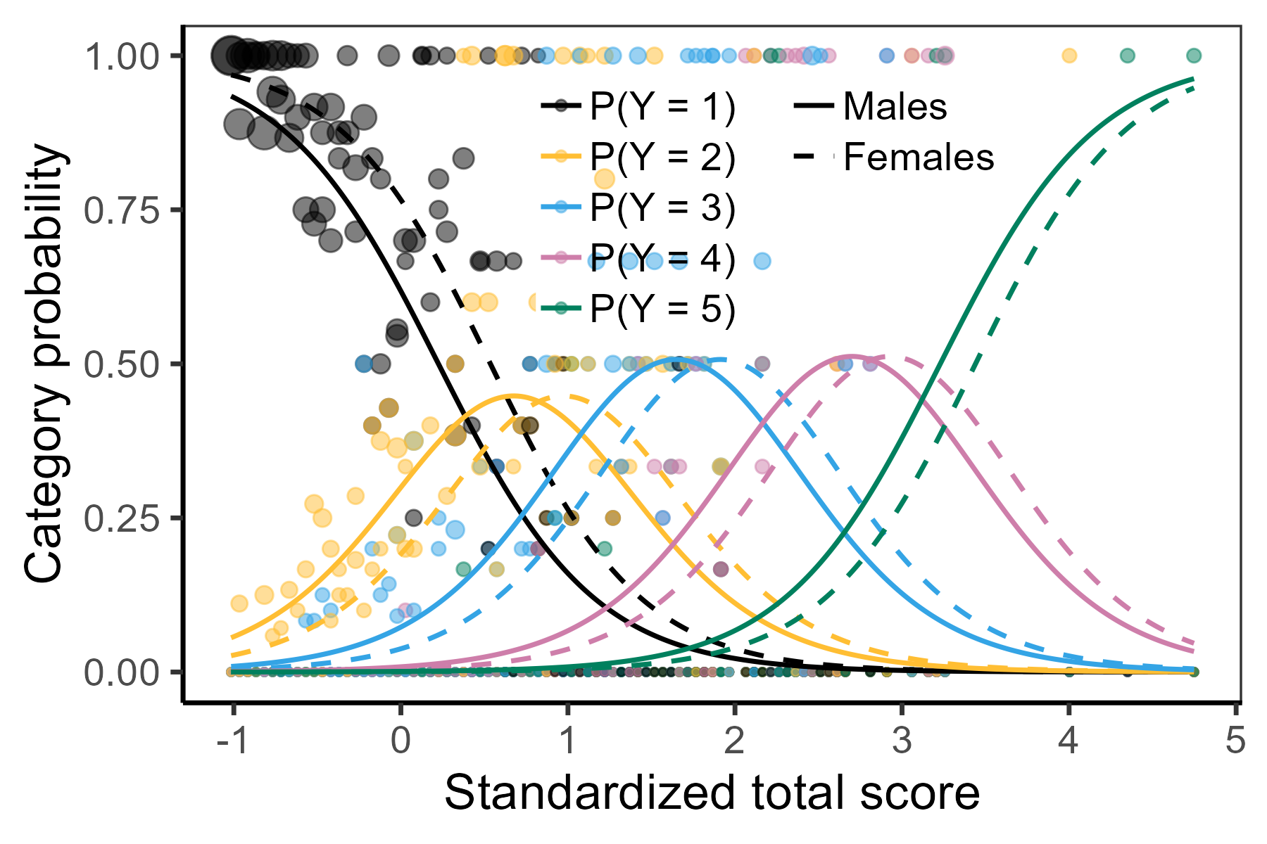
Anxiety dataset.
To be concerned about their mental health at least “sometimes” (category 2, blue lines in Figure 9.8 (a)) with a probability of 50%, males were estimated to have a level of anxiety 1.13 SD above average (see parameter b3) while a somewhat higher level of anxiety of 1.41 was shown for female respondents (see b3 + bDIF3). A similar trend can be observed for all categories, suggesting that males tend to worry about their mental health more often than females with the same overall level of anxiety (see also Figure 9.8 (b)).
The predict() method offers the computation of predicted values, i.e., category and cumulative probabilities for a given item and respondent with given matching criterion (anxiety level) and group membership specified via match and group arguments.
predict(fit_ORD1, item = "R6", match = 0, group = c(0, 1))
##   P(Y = 1) P(Y = 2) P(Y = 3) P(Y = 4)  P(Y = 5)
## 1   0.6179   0.2996   0.0729   0.0085    0.0010
## 2   0.7660   0.1915   0.0378   0.0042    0.0005
predict(fit_ORD1, item = "R6", match = 0, group = c(0, 1), type = "cumulative")
##   P(Y <= 1) P(Y <= 2) P(Y <= 3) P(Y <= 4) P(Y <= 5)
## 1         1    0.3821    0.0825    0.0095    0.0010
## 2         1    0.2340    0.0425    0.0047    0.0005
A respondent with an average level of anxiety, i.e., zero standardized total score, had a 30% probability of concerning about their mental health “sometimes” if they were males, while it was only 19% for females.
9.4.4 Group-specific adjacent category logit model
Another option to test for DIF in ordinal items is an extension of the adjacent category logit model Equation 6.22 which allows for model group-specific parameters. This model is preferred when we are interested in describing the ability needed to move from one category to the next one. The log-odds of the adjacent categories are modeled by a linear predictor including the ability matching criterion \(X_p\), the group membership variable \(G_p\), and their mutual interaction. More specifically, for an item \(i\) with \(K_i + 1\) ordinal categories we have
\[ \log\frac{\Pr(Y_{pi} = k|X_p, G_p)}{\Pr(Y_{pi} = k - 1|X_p, G_p)} = \beta_{i0k} + \beta_{i1} X_p + \beta_{i2} G_p + \beta_{i3} X_pG_p, \tag{9.13}\]
where \(k = 1, \dots, K_i\). Using a recursive formula (Exercise 9.5), it can be shown that category probability takes the following form:
\[ \Pr(Y_{pi} = k|X_p, G_p) = \frac{\exp\sum_{l = 1}^k \left(\beta_{i0l} + \beta_{i1} X_p + \beta_{i2} G_p + \beta_{i3} X_pG_p\right)}{1 + \sum_{j = 1}^{K_i} \exp\sum_{l = 1}^j \left(\beta_{i0l} + \beta_{i1} X_p + \beta_{i2} G_p + \beta_{i3} X_pG_p\right)}, \tag{9.14}\]
for \(k = 1, \dots, K_i\), while the category probability of the lowest category \(k = 0\) is computed as
\[ \Pr(Y_{pi} = 0|X_p, G_p) = \frac{1}{1 + \sum_{j = 1}^{K_i} \exp\sum_{l = 1}^j \left(\beta_{i0l} + \beta_{i1} X_p + \beta_{i2} G_p + \beta_{i3} X_pG_p\right)}. \tag{9.15}\]
The \(K_i\) parameters \(\beta_{i0k}\) are the \(k\) category-specific intercepts for the reference group within item \(i\). The slope parameters \(\beta_{i1}\) describe the effect of ability matching criterion \(X_p\) on the probability of gaining \(k\) points for the reference group in item \(i\). It is assumed to be the same for all categories. The parameter \(\beta_{i2}\) is associated with the effect of group membership variable \(G_p\), and it describes the difference in the intercept between the focal group and the reference group. Finally, the parameter \(\beta_{i3}\) is related to the effect of interaction between the ability matching criterion \(X_p\) and the group membership variable \(G_p\); i.e., it describes the difference in slope between the focal and the reference group. In total, we have \(K_i + 3\) parameters to estimate for item \(i\).
Estimation of item parameters and the DIF detection are analogous with the cumulative logit model described above, i.e., using the ML method (Section Section 6.5.2) and the LRT Equation 2.29.
IRT parametrization. Similarly, as in the previous models, the IRT parametrization may be applied to the adjacent category logit model for DIF detection Equation 9.13:
\[ \log\frac{\Pr(Y_{pi} = k|X_p, G_p)}{\Pr(Y_{pi} = k - 1|X_p, G_p)} = (a_{i} + a_{\text{DIF}i}G_p) \left(X_p - b_{ik} - b_{\text{DIF}ik}G_p\right), \tag{9.16}\]
which also applies to category probabilities Equation 9.14 and Equation 9.15 (Exercise 9.6). Parameters \(a_{i}\) and \(a_{\text{DIF}i}\) once again describe the slope of an IRC for the reference group and the difference in slope between the focal group and the reference group. However, interpretation of parameters \(b_{ik}\) and \(b_{\text{DIF}ik}\) is now related to the ability which is needed to move from category \(k - 1\) to category \(k\). In other words, \(b_{ik}\) is now the location of an intersection of related IRC for the reference group, and the term \(b_{ik} + b_{\text{DIF}ik}\) is the location of an intersection for the focal group.
The relationship between the two parametrizations is the same as it was for the cumulative logit models and a formula Equation 9.12 can be applied to switch between the parametrizations. Standard errors in the IRT parametrization can be calculated with the delta method Equation 6.10.
Group-specific adjacent category logit model with the difNLR package. In the difNLR package, the adjacent-category logit model can be utilized to test for DIF in ordinal items with the difORD() function, using the argument model = "adjacent". We again demonstrate the implementation of DIF detection with respect to gender using the Anxiety dataset. The output of the function once again summarizes LRT statistics and p-values.
(fit_ORD2 <- difORD(Data = Anxiety_items, group = Anxiety$gender,
                    focal.name = 1, model = "adjacent"))
## ...
##     Chisq-value P-value
## ...
## R6   9.8619      0.0072 **
## R7   9.9535      0.0069 **
## R8   1.0119      0.6029
## ...
## R19  9.1928      0.0101 *
## R20 11.1244      0.0038 **
## R21  3.0459      0.2181
## ...
## Items detected as DIF items:
## R6
## R7
## R19
## R20
As with the cumulative logit model, the adjacent-category model also identified, among others, item R6 “I was concerned about my mental health” to function differently for the two groups (\(LR\) = 9.86, df = 2, p-value = 0.01).
Estimates of item parameters for the final model can be again extracted using the coef() method, printed here with standard errors but without confidence intervals, and the IRCs can again be displayed using the plot() method.
coef(fit_ORD2, SE = TRUE, CI = 0)$R6
##              b2     b3     b4     b5      a
## estimate 0.6395 0.9013 2.1545 3.1694 1.3925
## SE       0.1119 0.1248 0.1905 0.3116 0.1205
##           bDIF2  bDIF3  bDIF4  bDIF5   aDIF
## estimate 0.2754 0.2677 0.2307 0.2008 0.0423
## SE       0.0900 0.0969 0.1745 0.2564 0.1274
plot(fit_ORD2, item = "R6", group.names = c("Males", "Females"))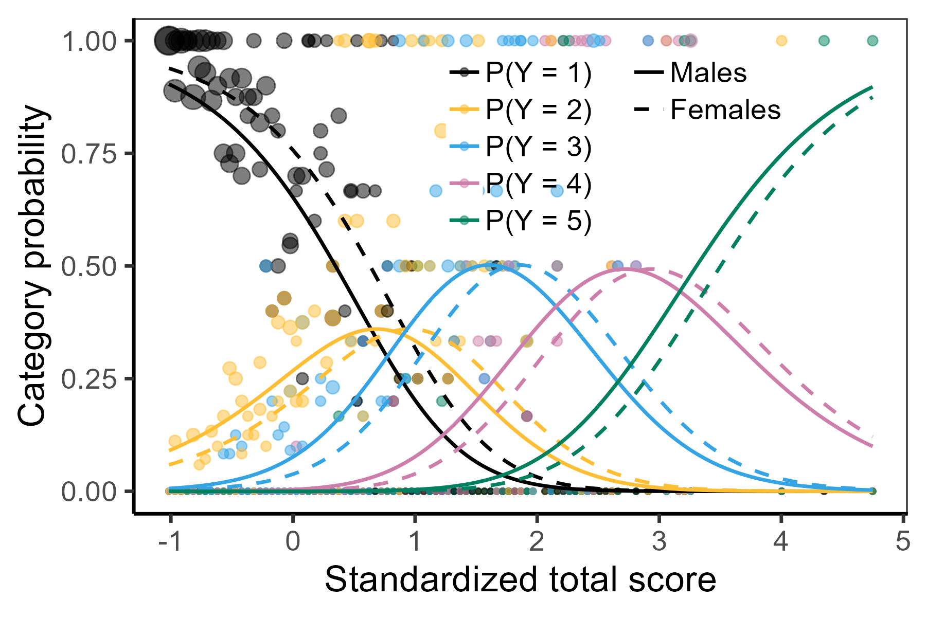
Anxiety dataset.
To move from category “rarely” to “sometimes” regarding a concern about their mental health, male respondents needed an Anxiety level (standardized total score) of 0.64 (SE = 0.12; see estimate of parameter b2) while female respondents needed an Anxiety level of 0.91 (see b2 + bDIF2), which corresponds to the locations of intersections between yellow and blue lines in Figure 9.9.
Method predict() can again be used to compute category probabilities for a given item and respondent with a given Anxiety level (matching criterion) and group membership specified via match and group arguments.
predict(fit_ORD2, item = "R6", match = 0, group = c(0, 1))
##   P(Y = 1) P(Y = 2) P(Y = 3) P(Y = 4)  P(Y = 5)
## 1   0.6522   0.2677   0.0763   0.0038   0.00005
## 2   0.7570   0.2037   0.0381   0.0012   0.00001
A male respondent with an average level of anxiety (match = 0) had a 65% probability of being concerned about their mental health “rarely”, while it was 75% for females with the same level of anxiety.
9.4.5 Group-specific multinomial regression model
To detect DDF among multiple-choice items, a group-specific extension of the multinomial regression model Equation 6.25 can be used. Consider that \(k = 0, \dots, K_i\) possible option choices are offered, with \(k = 0\) being the baseline category (such as the correct answer) and the other ones being distractors. The probability of option selection may differ between the reference group and the focal group. The multinomial model for DDF detection compares the probability of each response category \(k = 1, \dots, K_i\) with the probability of the baseline category \(k = 0\):
\[ \log\frac{\Pr(Y_{pi} = k|X_p, G_p)}{\Pr(Y_{pi} = 0|X_p, G_p)} = \beta_{i0k} + \beta_{i1k} X_p + \beta_{i2k} G_p + \beta_{i3k} X_pG_p. \tag{9.17}\]
In contrast to ordinal models Equation 9.11 and Equation 9.13, all parameters are category-specific and no ordering of the distractors is assumed. Parameters \(\beta_{i0k}\) are intercepts, and parameters \(\beta_{i1k}\) are slopes within item \(i\). Parameters \(\beta_{i2k}\) are associated with the effect of group membership on the probability of selecting option \(k\); in other words, they describe differences in intercepts between the focal group and the reference group when selecting option \(k\). Finally, parameters \(\beta_{i3k}\) are related to the effect of interactions between the group membership variable \(G_p\) and the matching criterion \(X_p\); i.e., they describe differences in slopes between the focal group and the reference group for category \(k\) in item \(i\). To sum up, the group-specific multinomial model for DDF detection Equation 9.17 includes \(4K_i\) item parameters for item \(i\) in total.
As with the adjacent category logit model for DIF detection Equation 9.13, using a recursive formula (Exercise 9.8), the probability of choosing a distractor \(k = 1, \dots, K_i\) is given by
\[ \Pr(Y_{pi} = k|X_p, G_p) = \frac{\exp\left(\beta_{i0k} + \beta_{i1k} X_p + \beta_{i2k} G_p + \beta_{i3k} X_pG_p\right)}{1 + \sum_{l = 1}^{K_i} \exp\left(\beta_{i0l} + \beta_{i1l} X_p + \beta_{i2l} G_p + \beta_{i3l} X_pG_p\right)}, \tag{9.18}\]
while the probability of the baseline category \(k = 0\) is added up to
\[ \Pr(Y_{pi} = 0|X_p, G_p) = \frac{1}{1 + \sum_{l = 1}^{K_i} \exp\left(\beta_{i0l} + \beta_{i1l} X_p + \beta_{i2l} G_p + \beta_{i3l} X_pG_p\right)}. \tag{9.19}\]
IRT parametrization. The IRT parametrization can again be applied in the multinomial model for DDF detection Equation 9.17:
\[ \log\frac{\Pr(Y_{pi} = k|X_p, G_p)}{\Pr(Y_{pi} = 0|X_p, G_p)} = (a_{ik} + a_{\text{DIF}ik}G_p) \left(X_p - b_{ik} - b_{\text{DIF}ik}G_p\right), \]
which results in category probabilities in the form of
\[ \Pr(Y_{pi} = k|X_p, G_p) = \frac{\exp(a_{ik} + a_{\text{DIF}ik}G_p)(X_p - b_{ik} - b_{\text{DIF}ik}G_p)}{1 + \sum_{l = 1}^{K_i} \exp(a_{il} + a_{il\text{DIF}}G_p)(X_p - b_{il} - b_{il\text{DIF}}G_p)}, \]
for \(k = 1, \dots, K_i\), while the baseline category probability is computed as
\[ \Pr(Y_{pi} = 0|X_p, G_p) = \frac{1}{1 + \sum_{l = 1}^{K_i} \exp(a_{il} + a_{il\text{DIF}}G_p)(X_p - b_{il} - b_{il\text{DIF}}G_p)}. \]
Parameters \(a_{ik}\) and \(a_{\text{DIF}ik}\) describe slopes of the IRCs for the reference group and the difference in slopes between the focal group and the reference group when selecting option \(k\). Parameters \(b_{ik}\) and \(b_{\text{DIF}ik}\) are, in contrast to an adjacent category logit model, now related to the ability which is needed to move from option \(k\) to baseline category \(0\), e.g., moving from distractor \(k\) to the correct answer.
The similar relationship as in Equation 9.12 can be used to recalculate between the two parametrizations, and the standard errors of estimates in IRT parametrization can be computed with the delta method Equation 6.10.
Group-specific multinomial regression model with the difNLR package. Testing for DDF under the multinomial regression model Equation 9.17 can be utilized with the ddfMLR() function in the difNLR package. Here we show the implementation of this function using the HCItest dataset which consists of 20 multiple-choice questions. We consider DDF detection with respect to the respondents’ gender using a standardized total score as the matching criterion. The ddfMLR() function allows us to specify the baseline categories with an argument key, in our case, the key for the correct answers HCIkey. Specifications of other inputs and arguments remain the same as in previously discussed functions of the difNLR or difR packages. Output summarizes the statistics of LRT and corresponding p-values.
data(HCItest, HCIkey, package = "ShinyItemAnalysis")

(fit_DDF <- ddfMLR(Data = HCItest[, 1:20], group = HCItest$gender,
                   focal.name = 1, key = HCIkey))
##         Chisq-value P-value
## ...
## Item.12 18.5029      0.0178 *
## Item.13  9.1026      0.1679
## ...
## Item.18  6.8674      0.3333
## Item.19 19.9421      0.0106 *
## Item.20 12.0779      0.0603 .
## ...
## Items detected as DDF items:
## Item.12
## Item.19
Items 12 (related to the set point temperature of the body) and 19 (related to the integrator – homeostatic system in the control center) were detected as those with differently functioning distractors for males and females (\(LR\) = 18.50 and 19.94, df = 8, p-values = 0.02 and 0.01 respectively).
Analogously to the ordinal models, the IRTpars argument can be used to choose between the IRT and classic intercept-slope parametrization in the coef() method. The estimated model parameters are now expressed with respect to the correct answer; no parameters are estimated for this category (category D in item 12 in the example below):
coef(fit_DDF, SE = TRUE)[[12]]
##                  b       a    bDIF    aDIF
## A estimate -2.0365 -1.0434  1.0564 -0.3526
## A SE        0.3755  0.2183  0.4323  0.3274
## B estimate -2.2219 -2.3621 -0.6212  1.3403
## B SE        0.2960  0.6244  1.3024  0.7707
## C estimate -2.6307 -1.0247  1.1059 -0.9152
## C SE        0.6225  0.2779  0.6715  0.4874
## E estimate -0.9933 -0.8399  0.4498 -0.3577
## E SE        0.1953  0.1385  0.2633  0.2436
plot(fit_DDF, item = 12, group.names = c("Males", "Females"))
Parameter b for option A is \(-2.04\) (SE = 0.38) which describes the standardized total score needed to move from selecting distractor A to choosing the correct answer D for male respondents, suggesting that this distractor was not very attractive. The term b + bDIF for category A is \(-0.98\) describing a standardized total score for female respondents, who seem to need a larger overall knowledge of homeostasis than males to choose the correct answer D over the distractor A (see the intersections between yellow and blue lines in Figure 9.10).
The predict() method can once again be used to obtain predicted probabilities of option selection. Here we display category probabilities in item 12 for both male and female students (group = c(0, 1)) of ability 1 SD below average (match = -1).
predict(fit_DDF, item = 12, match = -1, group = c(0, 1))
##        D      A       B     C      E
## 1 0.3863 0.1310 0.0216 0.0727 0.3885
## 2 0.2342 0.2408 0.0356 0.0846 0.4047
For a male respondent 1 SD below average, the probability of selecting the correct answer D is estimated to be 38.63%, while for a female respondent of the same ability, it is estimated at 23.43%. Female respondents at this ability level are estimated to more often select distractor A (with a probability of 24.08%) than their male peers of the same ability (13.10%).
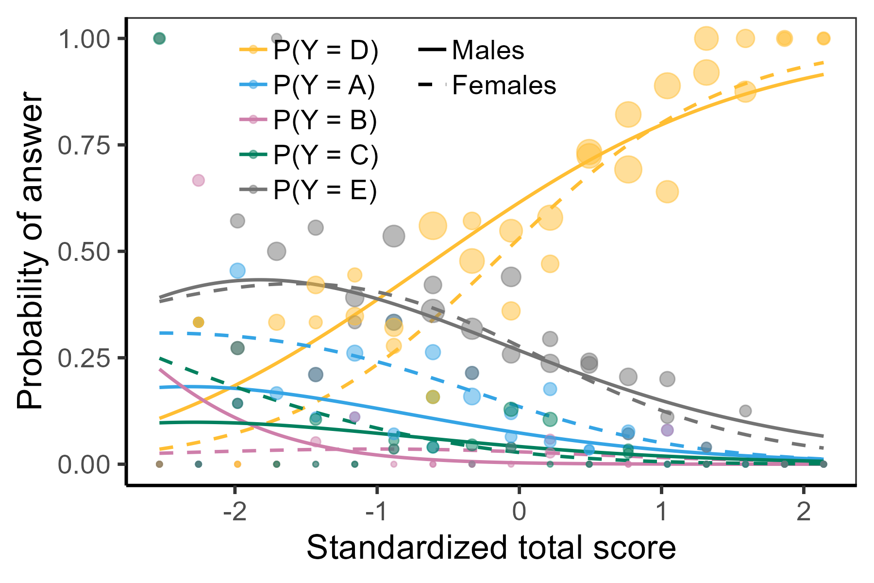
HCItest dataset.
9.5 IRT-based DIF detection methods
Similar to the regression models, the IRT models described in Chapter 7 and Chapter 8 can also be extended to account for multiple groups. Group-specific models are one of the extensions more generally studied within the exploratory IRT models, see De Boeck & Wilson (2004). Tests of submodels with constrained group-specific item parameters are then used to detect various types of DIF. We will first focus on group-specific IRT models. We will then describe the three most commonly used tests for DIF detection: Lord’s test, Raju’s test, and LRT.
9.5.1 Group-specific IRT models
Group-specific IRT models for testing DIF are latent variable models which are analogies to the regression models described in Section 9.4. The usual method is to fit two separate models, one for the focal group and one for the reference group, while estimated parameters are re-scaled (Candell & Drasgow, 1988; Lautenschiager & Park, 1988) (see also Section Section 10.3).
Group-specific IRT models in the difR package. In the difR package, the group-specific IRT models may be fitted with the function itemParEst() which allows for fitting the Rasch model and 1–3PL IRT models for binary data. It uses either the ltm or the lme4 package as an engine for estimating item parameters. It allows for fixing item discrimination and guessing parameters via arguments discr and c respectively.
Here we fit two models separately, one for males and one for females, for the MSATB dataset. Item parameters from the focal group (females) are then rescaled using equal means anchoring provided by the itemRescale() function (see also Section Section 10.3). Note that equal mean anchoring assumes balanced DIF. If this assumption is not met, this may lead to false results (see, for example, Kopf et al., 2015).
(fit_difR0 <- itemParEst(data = MSATB[MSATB$gender == 0, 1:20], model = "2PL"))
##             a       b  se(a)   se(b) cov(a,b)
## Item49 1.0404 -1.7197 0.1918  0.2600   0.0432
## Item27 1.1122  1.3154 0.1695  0.1812  -0.0235
## ...
## Item64 0.6661  0.0879 0.1240  0.1514  -0.0021
## ...
fit_difR1 <- itemParEst(data = MSATB[MSATB$gender == 1, 1:20], model = "2PL")
(fit_difR1 <- itemRescale(fit_difR0,fit_difR1))
##         new.a   new.b new.se(a) new.se(b) cov(a,b)
## Item49 0.9862 -2.3672    0.1518    0.2905   0.0406
## Item27 1.0462  1.2556    0.1143    0.1332  -0.0115
## ...
## Item64 0.4769  0.1196    0.0815    0.1480  -0.0021
## ...
Item 49 was somewhat easier for female respondents (\(b = -2.37\), SE = 0.29) than for males (\(b = -1.72\), SE = 0.26). On the other hand, item 64 seems to have higher discrimination for the male respondents (\(a = 0.67\), SE = 0.12) than for the females (\(a = 0.48\), SE = 0.08).
Estimated ICCs can be plotted using the plotDIFirt() function from the ShinyItemAnalysis package directly onto a matrix of estimated parameters for both groups, which is created here by using the base rbind() function:
plotDIFirt(parameters = rbind(fit_difR0,fit_difR1), item = 1)
plotDIFirt(parameters = rbind(fit_difR0,fit_difR1), item = 2)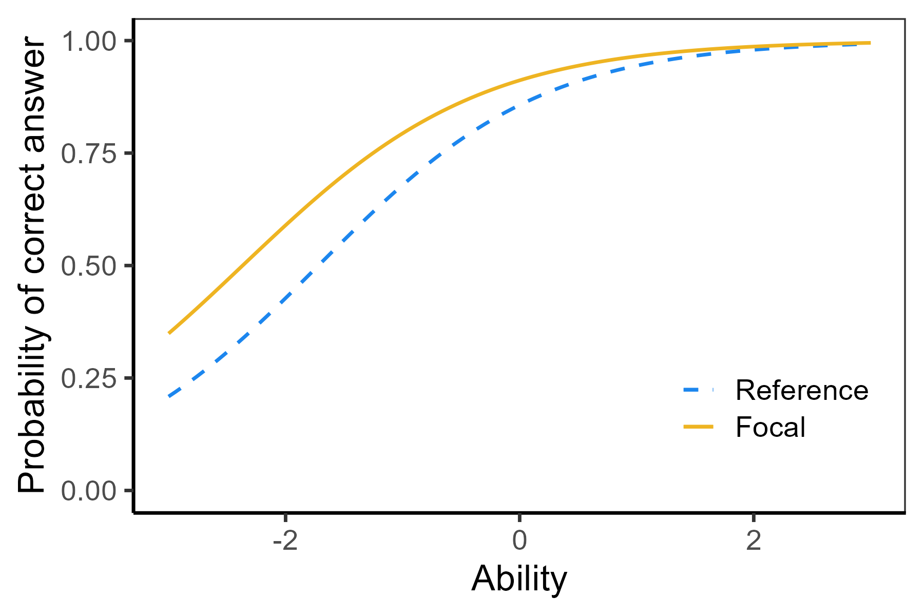
MSATB dataset.
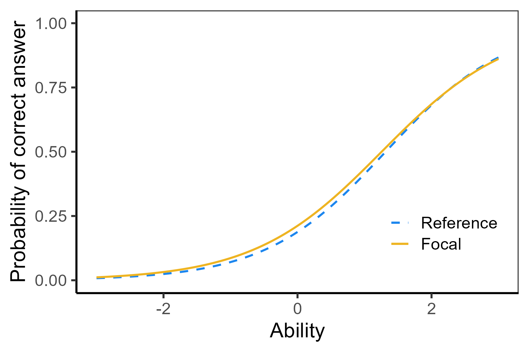
MSATB dataset.
ShinyItemAnalysis package.
As we noted above, there is a difference in difficulty for item 49 (Figure 9.11 (a)) while there are no large differences in estimated parameters for item 27 (Figure 9.11 (b)).
Group-specific IRT models in the mirt package. In the mirt package, the IRT models, which account for multiple groups, can be defined and fitted with the multipleGroup() function. As a default, the one-factor 2PL model is fitted. Higher-dimension models can be obtained by specifying the argument model (see also Section Section 8.3). Different item types may be specified with the argument itemtype, including ordinal and nominal models (see also Section Section 8.2).
Here we use the multipleGroup() function to fit two models separately for the males and females from the MSATB dataset as was done above. Alternatively, one may use the mirt() function for two subsets as in the difR package (see Supplementary R code). To extract estimated item parameters, we use the coef() method with arguments simplify = TRUE and IRTpars = TRUE to get a matrix of values in the IRT parametrization (see Section Section 7.2.2.1 for more details about coef() options in the mirt package).
fit_mirt0 <- mirt(MSATB[MSATB$gender == 0, 1:20], model = 1, SE = TRUE)
fit_mirt1 <- mirt(MSATB[MSATB$gender == 1, 1:20], model = 1, SE = TRUE)

fit_mirt <- multipleGroup(data = MSATB[, 1:20], model = 1,
                          group = as.factor(MSATB$gender), SE = TRUE)
coef(fit_mirt, simplify = TRUE, IRTpars = TRUE)
## $`0`
## $items
##             a       b g u
## Item49 1.0400 -1.7199 0 1
## Item27 1.1122  1.3156 0 1
## ...
## Item64 0.6659  0.0882 0 1
## ...
## $`1`
## $items
##             a       b g u
## Item49 0.9983 -2.3052 0 1
## Item27 1.0586  1.2746 0 1
## ...
## Item64 0.4826  0.1520 0 1
## ...
Estimated parameters are similar to those estimated by the estimPar() function from the difR package.
The ICCs can be plotted using the itemplot() function applied on the output of the multipleGroup() function. This time we plot ICCs of items 49 and 64.
itemplot(fit_mirt, item = "Item49")
itemplot(fit_mirt, item = "Item64")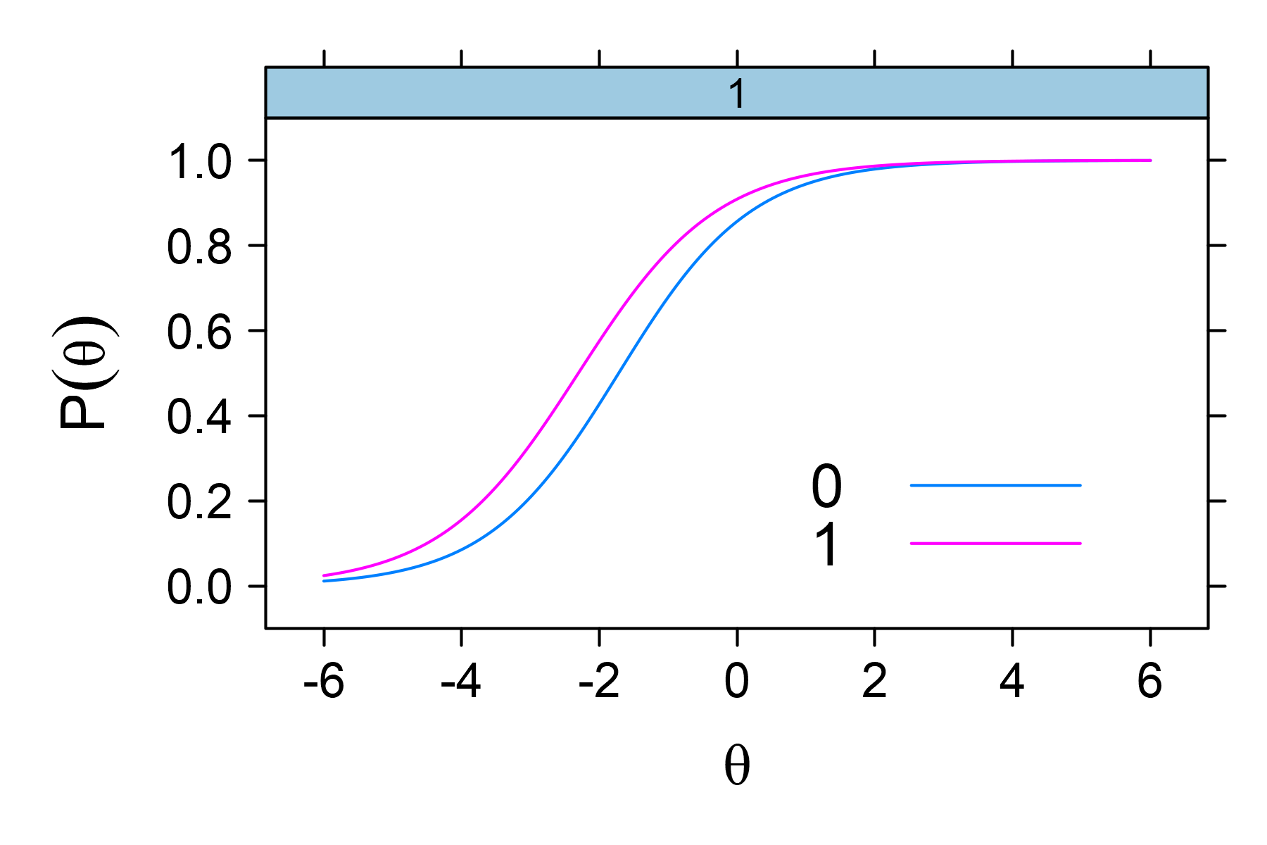
MSATB dataset.
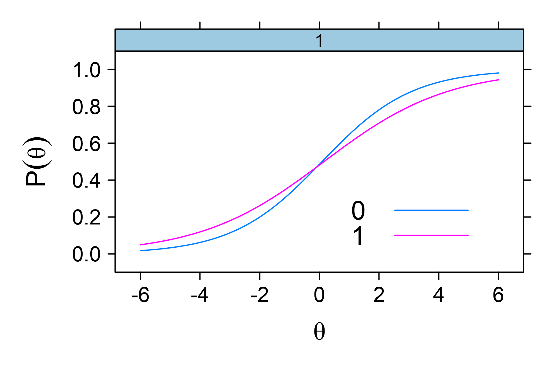
MSATB dataset.
mirt package.
Between-group differences in difficulties can once again be observed for item 49 (Figure 9.12 (a)). In item 64, the discrimination seems to differ for the two groups (Figure 9.12 (b)).
9.5.2 Lord’s test
The Lord’s test (Lord, 1980) is one of the most popular methods for testing DIF within the IRT framework. It uses a statistic of Wald’s type, similar to the statistic Equation 9.8, this time using the vector of the estimated differences in parameters between the reference and the focal group, and the estimate of a related covariance matrix. The corresponding test statistic \(W_i\) for item \(i\) has the following form:
\[ W_i = (\hat{\boldsymbol{\xi}}_{i0} - \hat{\boldsymbol{\xi}}_{i1})^\top \left(\hat{\mathbb{V}}_{i0} + \hat{\mathbb{V}}_{i1}\right)^{-1} (\hat{\boldsymbol{\xi}}_{i0} - \hat{\boldsymbol{\xi}}_{i1}), \tag{9.20}\]
where \(\hat{\boldsymbol{\xi}}_{i0}\) are estimated item parameters of the reference group, \(\hat{\boldsymbol{\xi}}_{i1}\) are estimated item parameters of the focal group, and \(\hat{\mathbb{V}}_{i0}\) and \(\hat{\mathbb{V}}_{i1}\) are the corresponding estimated covariance matrices (see Lord, 1980, p. 223).
Under the null hypothesis of no DIF, i.e., equal item parameters in both groups, the test statistic \(W_i\) has an asymptotic \(\chi^2\) distribution with as many degrees of freedom as there are item parameters (see Section Section C.2.2). When considering the 4PL IRT model, then \(\hat{\boldsymbol{\xi}}_{i0} = (\hat{a}_{i0}, \hat{b}_{i0}, \hat{c}_{i0}, \hat{d}_{i0})\) and \(\hat{\boldsymbol{\xi}}_{i1} = (\hat{a}_{i1}, \hat{b}_{i1}, \hat{c}_{i1}, \hat{d}_{i1})\) and \(W_i \stackrel{\text{as.}}{\sim} \chi^2_4\).
Lord’s test in the difR package. In the difR package, the Lord’s test is implemented with the difLord() function, in which the user can either provide estimated item parameters via the irtPar argument or just specify data, group variable, and name of the focal group as was shown in previously described functions of the difR package. Moreover, the user needs to specify which model should be fitted via the model argument. When estimated item parameters are provided, their matrix needs to take the form of output in the estimPar() function which was described above. Moreover, it is necessary to specify whether or not item parameters are on the same scale via the same.scale argument. In the latter case, the difR package offers re-scaling performed by equal means anchoring (Cook & Eignor, 1991). We show here both approaches of inputs, with both yielding the same results (see Supplementary R code). Output summarizes Lord’s statistics with their p-values.
difLord(irtParam = rbind(fit_difR0,fit_difR1), same.scale = TRUE)
difLord(Data = MSATB, group = "gender", focal.name = 1, model = "2PL")
## ...
##          Stat.  P-value
## Item49 9.5230 0.0086  **
## Item27 0.7242 0.6962
## ...
## Item64 1.6259 0.4436
## ...
## Detection threshold: 5.992 (significance level: 0.05)
## Items detected as DIF items:
##   Item49
The Lord’s test using the 2PL IRT model identified item 49 as functioning differently in the MSATB dataset (\(W\) = 9.52, df = 2, p-value = 0.01), which was probably caused by a difference in the difficulty parameter which was identified in Section 9.5.1 (Figure 9.11 (a) and Figure 9.12 (a)).
Lord’s test in the mirt package. In the mirt package, DIF is tested using the function DIF() applied to the output of the multipleGroup() function described above, and by then specifying which parameters are to be inspected for DIF. When both the slope a1 and the intercept parameters d are included, presence of any DIF is tested. Additionally, testing for uniform DIF can be enforced using the Rasch model and the DIF() function with the argument which.par = "d". The Lord’s test is available using the argument Wald = TRUE. Output summarizes Lord’s statistics, number of degrees of freedom, and corresponding p-values.
DIF(MGmodel = fit_mirt, which.par = c("a1", "d"), Wald = TRUE)
##             W df      p
## Item49 9.3335  2 0.0094
## Item27 0.4094  2 0.8149
## ...
## Item76 7.7364  2 0.0209
## ...
## Item64 1.5297  2 0.4654
## ...
## Item68 6.4863  2 0.0390
## ...
As with the previously described methods, the first item was observed to be functioning differently for males and females. Moreover, items 76 and 68 were also detected as DIF items, despite their p-values being regarded as non-significant, although borderline, when using the difLord() function from the difR package. Small differences between outputs of the two functions may be the result of different estimating methods and different scaling approaches applied in the two packages.
Note that, in contrast to the regression models in Section 9.4, ICCs differ even in a case when an item does not function differently (Figure 9.11 (b) and Figure 9.12 (b)). This is caused by fitting two separate models for the two groups.
Lord’s test in the equateIRT package. Another implementation of the Lord’s test can be found in the equateIRT package, which otherwise focuses on IRT equating methods (see Section Section 10.3). As was mentioned at the beginning of this section, re-scaling to a common scale is involved in a usual approach to group-specific IRT models. The dif.test() function of the equateIRT package offers more precise conversion of the item parameters to a common scale and intercept-slope parametrization to improve type I error rates of the Lord’s test (Battauz, 2019).
In our practical demonstration, we first extract estimated item parameters and covariance matrices from the group-specific models fitted by the mirt package, separately on the responses from males and females in the MSATB dataset. We then apply the dif.test() function to perform the Lord’s test for DIF detection between genders.
est0 <- import.mirt(fit_mirt0, display = FALSE)
est1 <- import.mirt(fit_mirt1, display = FALSE)

coefs <- list(est0$coef, est1$coef)
vars <- list(est0$var, est1$var)

dif.test(coef = coefs, var = vars)
## ...
##        statistic p.value
## ...
## Item49    12.149  0.0023 **
## Item61     2.906  0.2338
## Item64     1.859  0.3948
## Item68     5.890  0.0526 .
## ...
## Item76     6.228  0.0444 *
## ...
When using the default mean-mean equating method (Marco, 1977), items 49 and 76 were detected as functioning differently for males and females (\(W\) = 12.15 and 6.23, df = 2, p-values = 0.01 and 0.04, respectively).
9.5.3 Likelihood-ratio test
Another option for testing a group-free IRT submodel is to apply one of the most widely used tests in statistics – LRT (Thissen et al., 1988, 1993). Analogously to the non-IRT regression models, it is based upon the idea of assessing the goodness of fit for two competing models, one being a constrained version of the other, and using the ratio of their likelihoods given the observed data. If the constrained model is supported, the difference between their two likelihoods should be small, i.e., their ratio should be close to 1; in other words, the difference of the log-likelihoods should be close to 0.
The test statistic Equation 2.29 was shown to asymptotically follow the \(\chi^2\) distribution even in the IRT framework with degrees of freedom equal to the difference in the number of free parameters in the two nested models (Wilks, 1938).
Likelihood-ratio test in the mirt package. In the mirt package, DIF detection with the LRT can be utilized with the DIF() function by setting the argument Wald = FALSE. Analogously to the case of the Lord’s test, the DIF() function uses the output of the multipleGroup() function of the same package. Output now summarizes convergence status, information criteria such as AIC or BIC, and LRT statistics with number of degrees of freedom and p-values.
DIF(MGmodel = fit_mirt, which.par = c("a1", "d"), Wald = FALSE)
##        conv.    AIC    AICc   SABIC      HQ    BIC     X2 df      p
## Item49 TRUE -5.2880 -4.7943 -1.1428 -1.3644  5.210 9.2880  2 0.0096
## Item27 TRUE  3.5850  4.0786  7.7301  7.5085 14.083 0.4150  2 0.8126
## ...
## Item76 TRUE -3.5112 -3.0176  0.6339  0.4123  6.987 7.5112  2 0.0233
## ...
## Item64 TRUE  2.4286  2.9222  6.5737  6.3521 12.927 1.5714  2 0.4558
## ...
## Item68 TRUE -2.6954 -2.2018  1.4497  1.2281  7.803 6.6954  2 0.0352
## ...
Items 49, 68, and 76 were detected as functioning differently for the two groups, as was the case when using the Lord’s test with the mirt package.
9.5.4 Raju’s test
The Raju’s test is based upon an estimation of the area between the ICCs for the two groups. This method is only applicable for IRT models in which the asymptotes are the same for the two groups. This holds true for the Rasch and the 1–2PL IRT models; however, this method is also applicable for the 3PL and 4PL models in which the asymptotes do not differ between groups; otherwise the corresponding area is infinite (Raju, 1988).
In his work, Raju (1988) distinguished between the signed area and the unsigned area. In the case of a signed area, parts of the area are counted as positive when the ICC takes larger values for the reference group than for the focal group (vertical hatching in Figure 9.13 (a) and Figure 9.13 (b)); otherwise the area is counted as negative (horizontal hatching in Figure 9.13 (b)). In the case of an unsigned area, the absolute value of parts is considered (vertical hatching in Figure 9.13 (c)).
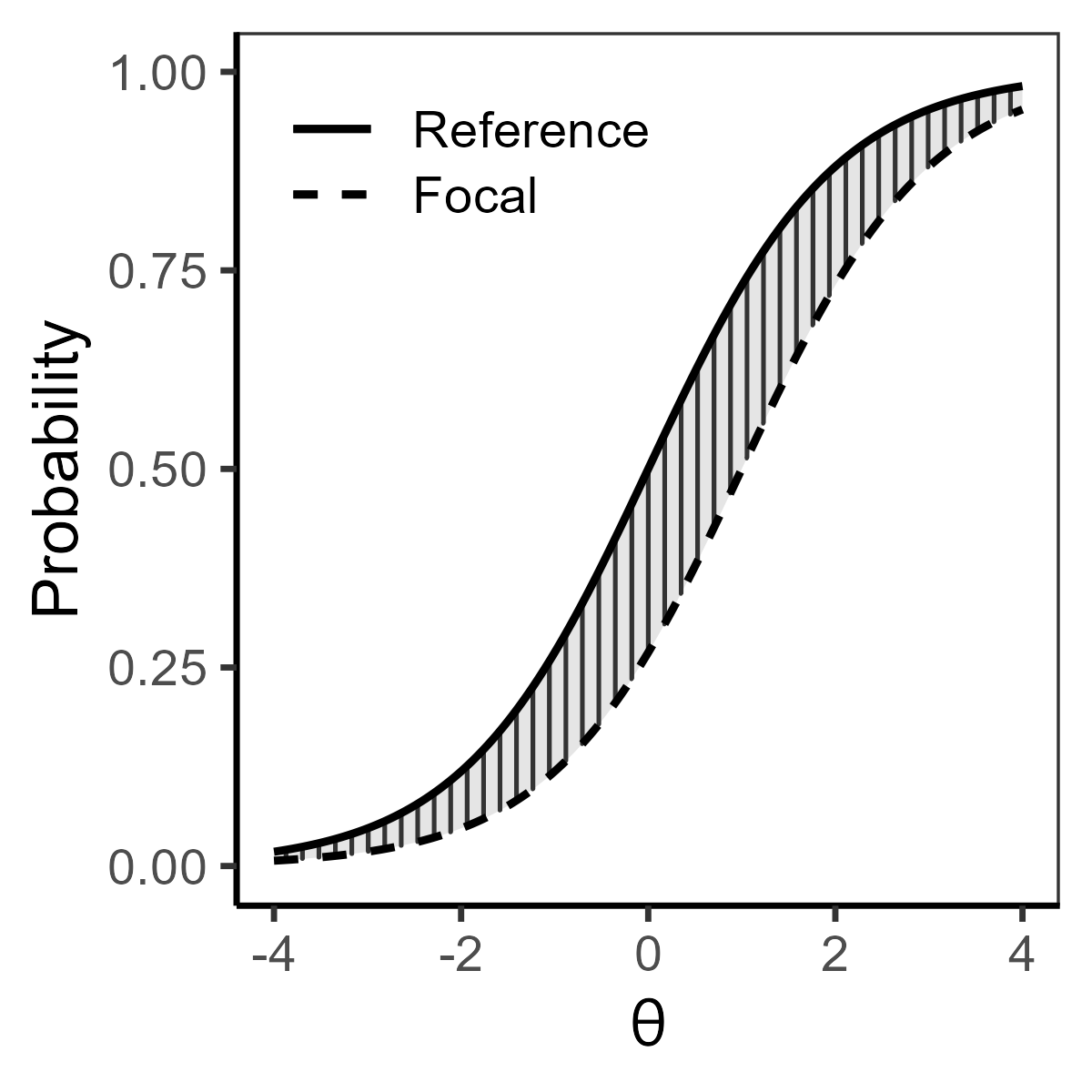
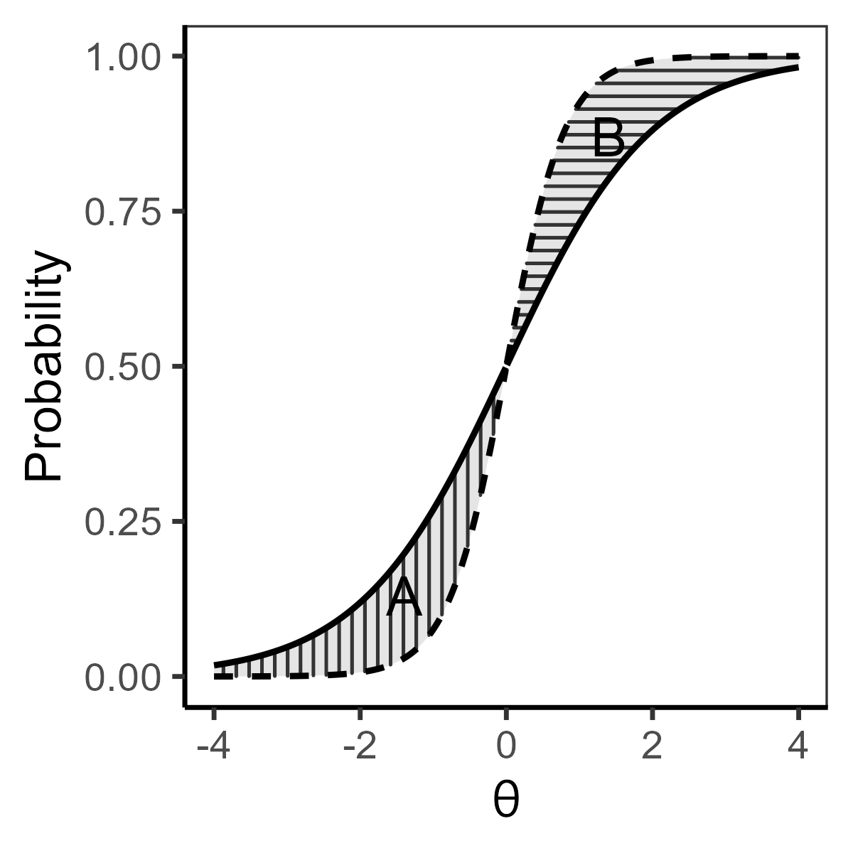
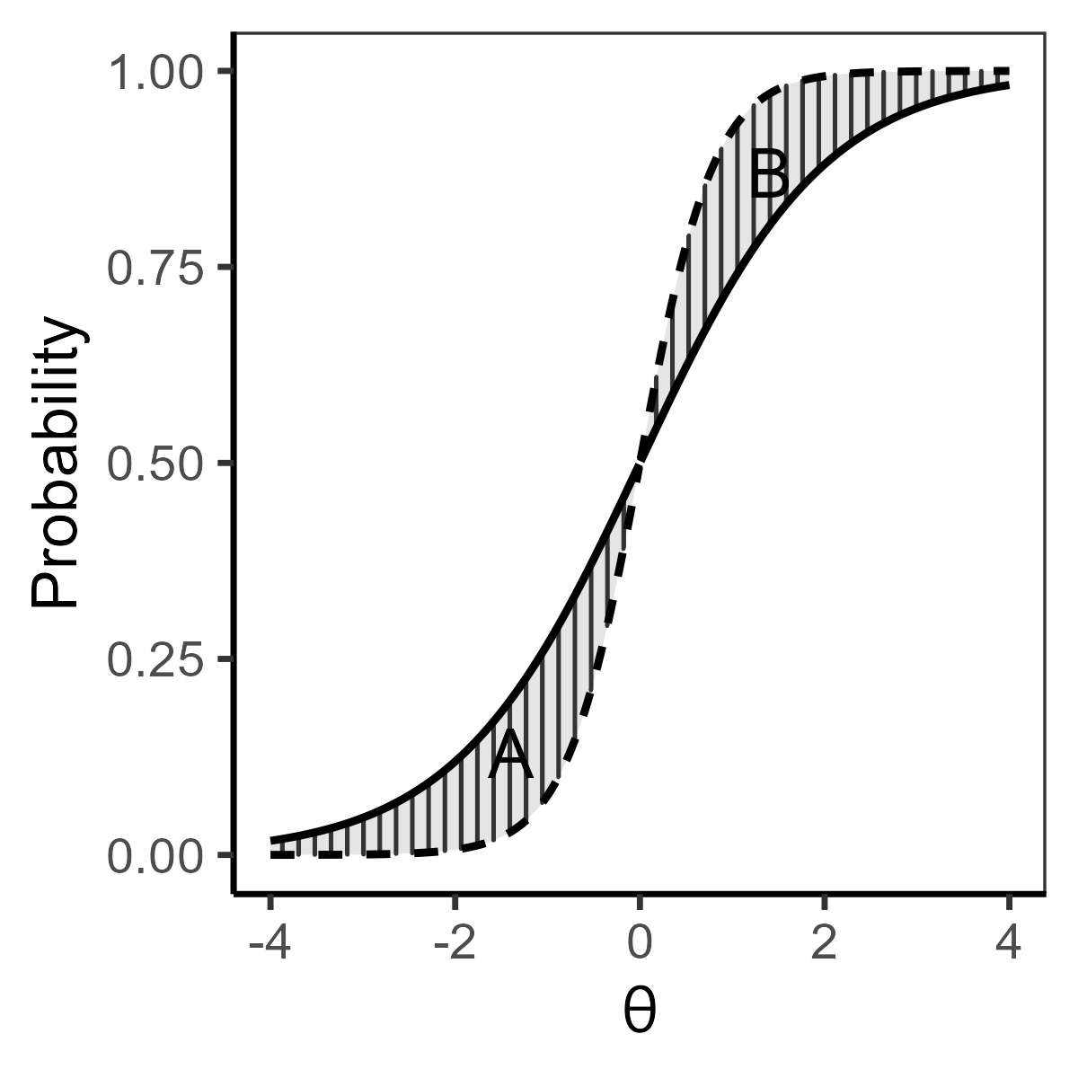
When considering the 4PL IRT model Equation 7.6 for both of the groups with the same values of the asymptotes (i.e., \(c_{i0} = c_{i1} = c_i\) and \(d_{i0} = d_{i1} = d_i\), where index 0 refers to the reference group and index 1 to the focal group), the signed area for item \(i\) is given as
\[ \text{SA}_i = (d_i - c_i)(b_{i1} - b_{i0}); \]
see Raju (1990) for proof. The signed area is based only upon the difference between difficulty parameters and the difference between upper and lower asymptotes which are the same for both groups, and it is not affected by the difference in discrimination parameters (Figure 9.13 (a) and Figure 9.13 (b)). It may even be the case that it is nearly zero, suggesting no DIF, when the difficulty parameters are the same for both groups while there is still a difference in discriminations (Figure 9.13 (b)). Therefore, a signed area may not be suitable to detect a non-uniform DIF.
On the other hand, the unsigned area (Raju, 1990) is given as
\[ \text{UA}_i =\, (d_i - c_i)\left|\frac{2(a_{i1} - a_{i0})}{Da_{i1}a_{i0}} \log\left(1 + \exp\left(\frac{Da_{i1}a_{i0}(b_{i1} - b_{i0})}{a_{i1} - a_{i0}}\right)\right) - (b_{i1} - b_{i0})\right| = (d_i - c_i)\left|R_i\right|, \]
where \(D = 1.702\) is the scaling constant. The unsigned area takes into account a difference in discrimination parameters and may be useful for detection of a non-uniform DIF (Figure 9.13 (c)).
The null hypothesis assumes that the true area is zero; i.e., the ICCs are identical and, therefore, there is no DIF (Raju, 1988, 1990). Considering the signed area \(\text{SA}_i\), the test statistic for item \(i\) is given as
\[ Z_i = \frac{\text{SA}_i - 0}{\sigma(\text{SA}_i)}, \tag{9.21}\]
where \(\sigma(\text{SA}_i)\) is a standard deviation of the signed area. It asymptotically follows a standard normal distribution and can be used in assessing the significance of an observed area between the two ICCs. Note that, when assuming the 1PL IRT model, the square of the Raju’s test statistic Equation 9.21 is identical to the Lord’s test statistic Equation 9.20.
Considering the unsigned areas \(\text{UA}_i\), distribution of \(|R_i|\) is half-normal; therefore it may be suitable to use
\[ Z_i = \frac{(d_i - c_i)R_i - 0}{\sigma\left((d_i - c_i)R_i\right)}, \]
with \(\sigma\left((d_i - c_i)R_i\right)\) being a standard deviation of \(\left((d_i - c_i)R_i\right)\), which has an asymptotically normal distribution (Raju, 1990).
Area between two ICCs in the DFIT package. The DFIT package implements two functions to compute the signed and unsigned area between two ICCs – SignedArea() and UnsignedArea(). For both functions, it is necessary to prepare a list of estimated parameters for the reference and focal groups and to specify an underlying IRT model. For the UnsignedArea() function, one needs to choose whether to keep the scaling constant \(D = 1.702\) with an option logistic = FALSE or whether to replace it by 1 with logistic = TRUE. However, calculation of the area between the ICCs from the formulae for \(SA_i\) and \(UA_i\) provided above is straightforward and easy to implement even in base R (see Supplementary R code).
In the example below, we compute the signed and unsigned areas for items of the MSATB dataset using the previously estimated item parameters of the 2PL IRT model using the difR package (saved outputs fit_difRO and fit_difR1).
library(DFIT)
itemPar <- list(reference = fit_difR0[, 1:2],  focal = fit_difR1[, 1:2])
SA <- SignedArea(itemParameters = itemPar, irtModel = "2pl")
UA <- UnsignedArea(itemParameters = itemPar, irtModel = "2pl", logistic = FALSE)
cbind(SA, UA)
##             SA     UA
## Item49  0.6475 0.6475
## Item27  0.0598 0.0701
## ...
## Item64 -0.0317 0.4858
## ...
For item 49, the signed and unsigned areas are almost the same, which is to be expected given that the difference between its estimated discrimination parameters is negligible while the difference between its estimated difficulties is noticeable (Figure 9.11 (a) and Figure 9.12 (a)). For item 27, both areas are almost zero, given that the difference between the estimated item parameters and between the two ICCs is small (Figure 9.11 (b)). On the other hand, the signed area for item 64 is negligible while the unsigned area is \(0.49\) (Figure 9.12 (b)).
Raju’s test in the difR package. To test whether the signed or unsigned area is significantly different from 0, the Raju’s test can be utilized with the difRaju() function of the difR package. Specification of the inputs is analogous to previous functions for DIF detection in this package. An option for the signed area may be chosen by the signed = TRUE argument. We again use the MSATB dataset and the 2PL IRT model:
difRaju(Data = MSATB, group = "gender", focal.name = 1, model = "2PL",
        signed = TRUE)
##        Stat.   P-value
## Item49 -1.6608  0.0967 .
## Item27 -0.2659  0.7903
## ...
## Item64  0.1499  0.8809
## ...
difRaju(Data = MSATB, group = "gender", focal.name = 1, model = "2PL",
        signed = FALSE)
##        Stat.   P-value
## Item49 -1.6607  0.0968 .
## Item27 -0.6981  0.4851
## ...
## Item64 -1.3101  0.1902
## ...
## Item68 -2.2388  0.0252 *
## ...
When the signed area is considered, no item is detected to be functioning differentially between males and females. In the case of the unsigned area, item 68 is identified as a DIF item (\(Z = -2.24\), p-value = 0.03). In item 64, the absolute value of the test statistic is larger when considering the unsigned area; however, the area remains insignificant.
9.6 Other methods
There are plenty of other methods for DIF detection. Some extend existing procedures, for example, to account for multiple groups, for a type of DIF for which detection is suitable, or by incorporating an ability estimate yielded by another method.
9.6.1 Iterative hybrid ordinal logistic regression with IRT
The iterative hybrid ordinal logistic regression and IRT extends the DIF detection procedure based upon the cumulative logit model Equation 9.10 by using IRT-based ability estimates and by employing an iterative algorithm analogous to item purification. Ability estimates are based upon either a graded response model Equation 8.1 or another suitable ordinal IRT model, while appropriate equating technique needs to be applied (see Section Section 10.3). For detailed description of the algorithm, the reader is referred to Choi et al. (2011).
Iterative hybrid ordinal logistic regression with IRT in lordif package. Iterative hybrid ordinal logistic regression with IRT may be fitted using the lordif package and its lordif() function. We will illustrate the algorithm with the Anxiety dataset considering DIF detection with respect to gender of the respondents.
With the lordif() function, it is necessary to specify response data and the group membership variable via the resp.data and group arguments, respectively. Note that the default significance level is 0.01; we set argument alpha = 0.05 to change the significance level to 0.05 in order to get comparable results to previous methods. The output summarizes a number of categories in each item and \(\chi^2\) statistics of the LRT considering uniform DIF (slope chi12), any DIF (slope chi13), or non-uniform DIF (slope chi23).
library(lordif)
lordif(resp.data = Anxiety_items, group = Anxiety$gender, alpha = 0.05)
## ...
## Items flagged: 6, 7, 9, 10, 19, 20, 21, 29
## ...
##    item ncat  chi12  chi13  chi23
## 6     6    5 0.0000 0.0000 0.0524
## 7     7    4 0.0430 0.0043 0.0091
## 8     8    4 0.6301 0.7511 0.5595
## 9     9    4 0.0176 0.0408 0.3833
## 10   10    4 0.0206 0.0035 0.0145
## ...
## 19   19    4 0.0022 0.0077 0.5309
## 20   20    4 0.0183 0.0211 0.1425
## 21   21    4 0.0108 0.0389 0.9948
## ...
## 29   29    4 0.0120 0.0305 0.4144
The algorithm ended after two iterations detecting items R6, R7, and R10 as functioning differently for males and females in a non-uniform way, while items R9, R19, R20, R21, and R29 were flagged for uniform DIF. Item parameter estimates are saved in the ipar.sparse values of the output.
fit_lordif$ipar.sparse
##            a    cb1    cb2    cb3    cb4
## ...
## I6.1  2.3511 0.3619 1.1025 1.8668 2.6918
## I6.2  3.0226 0.6220 1.2403 1.9581 2.6711
As an example, there is a clear difference in discrimination for item R6 “I was concerned about my mental health”, while the cumulative logit model for DIF detection fitted on standardized total scores identified this item as functioning differently in a rather uniform way (see Section 9.4.3).
9.6.2 Regularization approach for DIF detection
So far we have focused on DIF detection based upon a single grouping variable. When several grouping variables are of interest, the respective DIF detection method is typically applied independently for each of these grouping variables. Another option is to use a regularization approach which considers all grouping variables simultaneously using a lasso-based method. For example, Tutz & Schauberger (2015) offered the Rasch model that includes multiple variables using the regularization approach (specifically a penalized maximum likelihood estimator) to identify DIF items.
However, the regularization approach has not been used only for identifying DIF considering multiple grouping variables. For example, Magis et al. (2015) proposed a method based upon a logistic regression model which is formulated for all item responses simultaneously, which improves upon testing item-by-item. Finally, Schauberger & Mair (2020) proposed a lasso-based method for the detection of uniform DIF using a broad range of polytomous IRT models which are also estimated using a penalized likelihood.
9.6.3 Measurement invariance: Factor analytic approach
The equivalence of the IRT and the factor analysis demonstrated in Section Section 7.5 can be generalized to account for grouping variables and other covariates. From this generalization, it follows that DIF tested within the IRT framework directly translates to the measurement invariance across groups tested within the confirmatory factor analytic framework. The differences are once again in the estimation approach of the models. For further comparison of the two approaches, see Raju et al. (2002) or Teresi (2006).
9.7 DIF detection in interactive application
Section DIF/Fairness in the ShinyItemAnalysis interactive application offers a number of tools for DIF detection. For non-IRT methods, DIF can be analyzed with respect to a (standardized) total score, as well as with respect to other external matching criteria, which can be uploaded separately in the Data tab.
The Scores tab provides descriptive statistics and a histogram for ability scores used as the matching criterion with respect to groups. If an external observed score is uploaded (such as the pre-test total score), selection between the total score and the uploaded matching variable is offered.
The Delta plot is offered under a tab of the same name. The user can choose either a fixed or a normal threshold. For selected settings, a diagonal plot is displayed with a summary table, which contains information about the proportions of correct answers in both the reference group and the focal group together with their transformations into delta scores, and with the distances of the delta scores from the main axis of the ellipse formed by the delta scores.
In the Mantel-Haenszel tab, the subtab Summary shows a summary table for the MH test, including test statistics, corresponding p-values, odds ratios, and their standardized forms. The Items subtab offers deeper insight into the way the MH statistic is constructed. Other traditional DIF detection methods provided by the ShinyItemAnalysis interactive application include the SIBTEST.
Regression models for DIF detection are implemented in a number of tabs and offer the logistic regression model Equation 9.5, generalized logistic regression model Equation 9.9, cumulative logit Equation 9.11, adjacent category logit Equation 9.14, and nominal category regression models Equation 9.17. Selection between IRT parametrization and classical intercept-slope parametrization is offered for each of these models. The user can further specify the DIF type to be tested and the matching criterion to be used. Within each of these tabs, the subtab Summary displays a summary table including information about the DIF test statistics, effect sizes, and parameters of all items included in the final model. The subtab Items offers IRC plots under the final model (see Figure 9.14 for the cumulative logit regression model).
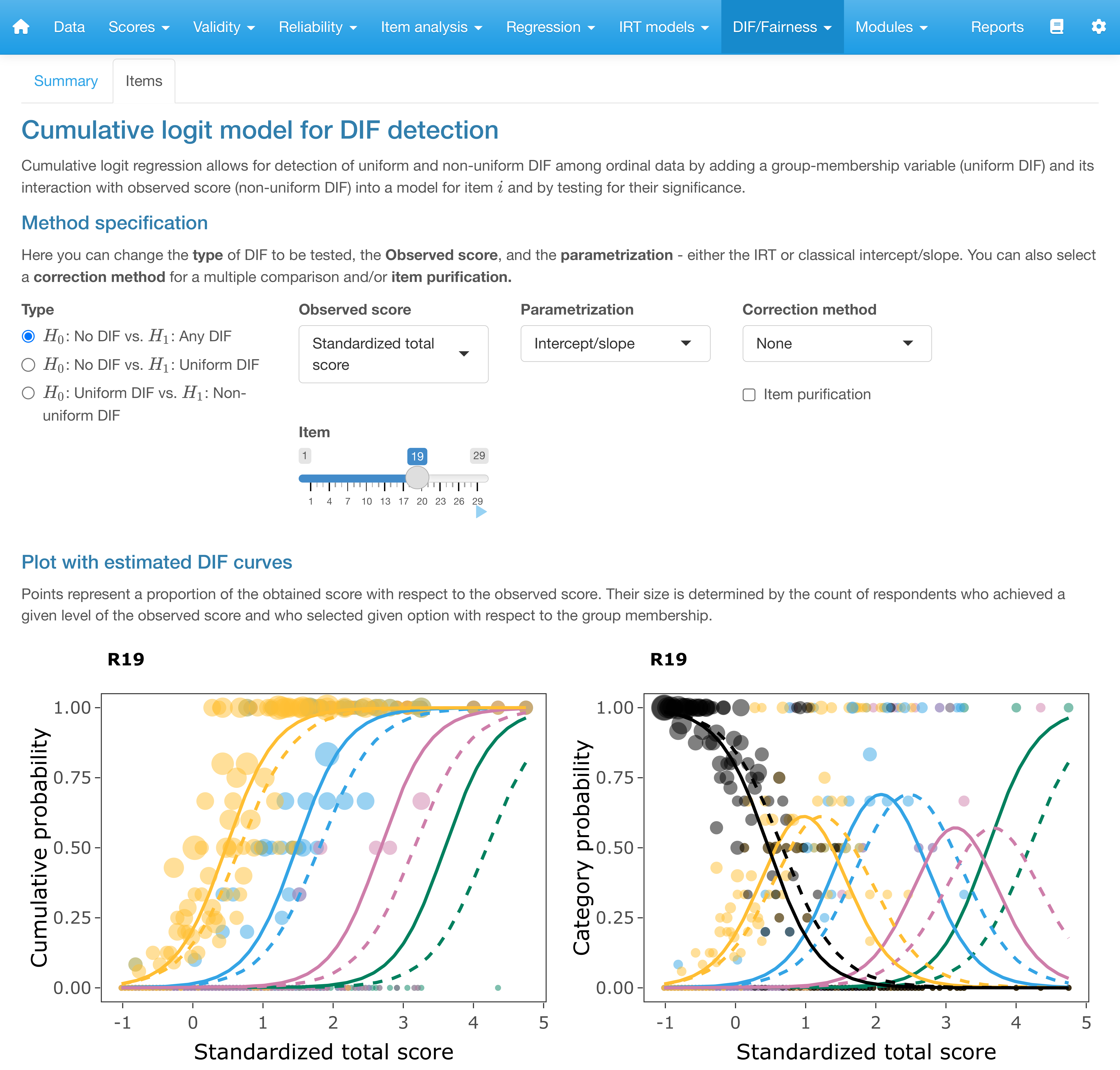
ShinyItemAnalysis.
DIF detection under the binary IRT models (1PL, 2PL, and 3PL with the same guessing parameter for the two groups) is implemented with the Lord’s test Equation 9.20 and the Raju’s test within the tabs of the same names. Also within these tabs, the subtab Summary offers a summary table for all items, while the subtab Items displays plots of ICCs using the larger model.
Finally, method comparison is provided for DIF detection methods (for binary items only). The application also includes a training section with interactive exercises. As always, a sample R code can be used to try analyses in R.
9.8 Summary
In this chapter, we have introduced methods for testing between-group differences on the item level with various DIF and DDF detection methods. We started with traditional approaches, including the Angoff’s Delta plot method, MH test, and SIBTEST. We then discussed procedures based on regression models, for binary, ordinal, and nominal items. We have subsequently focused on IRT-based DIF detection methods and on other methods. Practical examples were presented with the deltaPlotR, difR, difNLR, equateIRT, and mirt packages, as well as within the interactive ShinyItemAnalysis application.