5 Traditional Item Analysis
5.1 Introduction
Previous chapters focused on the measurement instrument as a whole, especially upon its reliability and validity. However, the quality of a multi-item instrument is always dependent upon the quality of its items. Item-level analysis may provide a deeper insight into the properties of individual items and more informed decisions about their revision.
In this chapter, we will first describe the main traditional item characteristics including item difficulty and item discrimination. We will provide graphical tools for a traditional description of item functioning and the functioning of individual distractors. We will also discuss how reliability and validity may be analyzed on the item level and used for item selection to maximize instrument reliability and validity, or how analysis of missed items may provide useful information for adjusting the test length.
Traditional item analysis uses counts, proportions, and correlations to evaluate the properties of test items. It offers tools that are easily applicable and easily calculated, oftentimes even by hand. The methods presented here assume unidimensional latent trait, and as such are inappropriate when the construct is explicitly multidimensional. These tools may be understood as empirical counterparts and prerequisites for more complex item functioning descriptions based on regression and IRT models which will be discussed in Section 9.4 and Chapter 7 and Chapter 8.
5.2 Item difficulty
Assessing item difficulty/popularity is important for practical reasons. In educational but also other contexts, providing some easy items at the beginning of the test may help increase respondent confidence and lower test anxiety. The range of item difficulties typically differs with respect to the purpose of the test. In a criterion-referenced test it is expected that many students will answer most of the items correctly. Contrarily, in a norm-referenced test and especially in high-stakes educational tests, the test needs to contain a higher number of difficult items in order to distinguish between the strongest test takers.
In binary items, a natural estimate of item difficulty is the proportion of respondents who answered that item correctly. In ordinal items, a difficulty estimate can be more generally based on the average item score. In the context of educational testing, a higher average item score is obtained in the case of easier items; thus a more precise term would be item easiness or item facility, but difficulty is historically more common. In psychological or health-related measurements, the correct answer, sometimes termed the key answer, is considered an answer which counts towards the measured trait, and the item difficulty is the popularity of this correct answer – that is the ratio of respondents who chose (endorsed) this answer. Keeping this in mind, later in this text, we will use the terms correct answer and item difficulty also in contexts other than educational testing.
5.2.1 Difficulty in binary items
In binary items, difficulty is traditionally estimated as the ratio \(\hat{\pi}_i\) of respondents who answered item \(i\) correctly. This is equivalent to the average item score \(\bar{Y}_{\bullet i}\):
\[ \hat{\pi}_i = \bar{Y}_{\bullet i} = \frac{1}{n}\sum_{p = 1}^n Y_{pi}. \tag{5.1}\]
It should be noted that a traditional estimate of item difficulty is sample dependent; i.e., it depends upon the ability or level of the latent trait of the respondents. For example, in the context of educational testing, an item may appear difficult to a group of low ability students, while it may appear easy to a group of high ability students. This issue is partly solved within the framework of regression and IRT models.
In binary items, the sample variance of the item score is simply \(\hat{\pi}_i (1 - \hat{\pi}_i)\); thus the sample standard deviation is
\[ s_i = \sqrt{\hat{\pi}_i (1 - \hat{\pi}_i)}, \tag{5.2}\]
both fully determined by the average score and reaching the maximum for items with difficulty of \(\hat{\pi}_i = 0.5\).
Difficulty in binary items in R. Traditional data analysis is demonstrated below on binary data of a 20-item HCI dataset. In R, estimate of item difficulty Equation 5.1 is easily accessible via the base mean() function. Joint enumeration for all items is provided by using the sapply() function.
data(HCI, package = "ShinyItemAnalysis")
sapply(HCI[, 1:20], mean)
##  Item 1  Item 2  Item 3  Item 4  Item 5  Item 6  Item 7  Item 8  Item 9 Item 10
##  0.6989  0.7527  0.8479  0.4040  0.4424  0.3625  0.5469  0.7051  0.4332  0.6482
## Item 11 Item 12 Item 13 Item 14 Item 15 Item 16 Item 17 Item 18 Item 19 Item 20
##  0.7788  0.5730  0.6083  0.7588  0.4439  0.6068  0.2965  0.7972  0.7849  0.7220
For example, item 3 was easy to answer, since the percentage of correct answers was almost 85%. On the other hand, item 17 was the most difficult in the test, being answered correctly by less than 30% of respondents.
Calculation of item standard deviations Equation 5.2 are implemented with the sd() function.
sapply(HCI[, 1:20], sd)
##  Item 1  Item 2  Item 3  Item 4  Item 5  Item 6  Item 7  Item 8  Item 9 Item 10
##  0.4591  0.4318  0.3594  0.4911  0.4971  0.4811  0.4982  0.4564  0.4959  0.4779
## Item 11 Item 12 Item 13 Item 14 Item 15 Item 16 Item 17 Item 18 Item 19 Item 20
##  0.4154  0.4950  0.4885  0.4281  0.4972  0.4888  0.4571  0.4024  0.4112  0.4484
The lowest standard deviation was observed, as expected, in item 3 with difficulty furthest from \(0.5\), while the highest standard deviation was observed in item 7 with difficulty closest to \(0.5\).
5.2.2 Difficulty in ordinal items
In ordinal items, the average item score \(\bar{Y}_{\bullet i}\) may again be used to estimate item difficulty. In order to obtain item difficulty indices comparable across all items in a multiple-item instrument (possibly scored on different scales), it may be helpful to scale each average item score to interval \([0, 1]\) by accounting for a minimal and maximal possible item score \(\text{min}(Y_i)\) and \(\text{max}(Y_i)\):
\[ \hat{\pi}_i = \frac{\bar{Y}_{\bullet i} - \text{min}(Y_i)}{\text{max}(Y_i) - \text{min}(Y_i)}. \tag{5.3}\]
The ordinal data may be dichotomized to calculate item difficulty. One way is to dichotomize by the maximal possible score \(\text{max}(Y_i)\), i.e., to estimate item difficulty as a ratio of those who reached the maximal item score:
\[ \hat{\pi}_i = \frac{1}{n}\sum_{p = 1}^n I(Y_{pi} = \text{max}(Y_i)). \tag{5.4}\]
Dichotomization of ordinal items may be generalized by using a cut-off value \(k_i\), in which case difficulty is estimated by the ratio of respondents who reached at least \(k_i\) points in that item:
\[ \hat{\pi}_i = \frac{1}{n}\sum_{p = 1}^n I(Y_{pi} \geq k_i), \tag{5.5}\]
where \(k_i\) may be the midpoint, the median, or any other pre-specified value.
Difficulty in ordinal items in R. For demonstration, we will use the Anxiety dataset, with Likert-scored items on a scale from 1 (never) to 5 (always). We will focus on item R25 “I had difficulty sleeping”. In R, the difficulty index for ordinal data estimated by mean item score can be easily calculated with the base mean() function.
data(Anxiety, package = "ShinyItemAnalysis")
mean(Anxiety[, "R25"])
## [1] 2.4047
sd(Anxiety[, "R25"])
## [1] 1.2124
The average score on item R25 is 2.40 with a standard deviation of 1.21.
Next, we compute the corrected item difficulty Equation 5.3:
(mean(Anxiety[, "R25"]) - 1) / (5 - 1)
## [1] 0.3512
Accounting for the maximal and minimal possible score, the corrected difficulty estimate for item R25 is 0.35.
For item R25 of the Anxiety dataset, we shall display difficulties of binarized items Equation 5.4 obtained using different cut-off values.
mean(Anxiety[, "R25"] >= 5)
# [1] 0.0561
mean(Anxiety[, "R25"] >= 4)
# [1] 0.1919
mean(Anxiety[, "R25"] >= 3)
## [1] 0.4661
mean(Anxiety[, "R25"] >= 2)
## [1] 0.6906
When binarizing the data in such a way that the answer was scored as 1 only when respondent always had difficulty sleeping and 0 otherwise, the difficulty is assessed at 0.06. Other dichotomizations lead to higher item difficulty.
Difficulty in the ShinyItemAnalysis package. Item difficulty estimates and more item characteristics are all jointly offered in the ItemAnalysis() function of the ShinyItemAnalysis package. Here we display only some columns of the output, namely the item difficulty Equation 5.3, item mean, item SD, observed minimum and maximum item score, and proportion of respondents who chose the maximal score Equation 5.4.
library(ShinyItemAnalysis)
Anxiety_items <- Anxiety[, paste0("R", 1:29)]
ItemAnalysis(Data = Anxiety_items)[, c("Difficulty", "Mean", "SD", "Min.score",
                                       "Max.score", "Prop.max.score")]

##      Difficulty  Mean      SD Min.score Max.score Prop.max.score
## R1       0.1230 1.4922 0.8303         1         5         0.0078
## ...
## R25      0.3512 2.4047 1.2124         1         5         0.0561
## ...
For item R25, the item difficulty of 0.35, mean of 2.40, SD of 1.21, and proportion of 0.05 of those who reached the maximal item score align with values obtained previously.
5.3 Item discrimination
Item discrimination describes an item’s ability to distinguish between respondents with a high and low level of a latent trait, e.g., between high and low ability students, highly and less impaired patients, or those with a high or low level of fatigue or pain.
The traditional discrimination indices are based on correlations between item and test scores, or differences in average scores between an upper and lower group of respondents. Note that these indices assume unidimensional latent trait, because they are calculated based on total score; thus they are inappropriate when the construct is explicitly multidimensional. Further limitations of these indices are again their sample-dependence, i.e., that they depend upon the homogeneity of respondents tested. For example, an item can appear well discriminating in a heterogeneous group and not-so-well discriminating in a homogeneous group of respondents. This weakness is to some extent solved in item discrimination estimates based upon regression and IRT models.
5.3.1 Correlation between item and total score
Item discrimination is traditionally estimated by the sample Pearson RIT (item-total correlation):
\[ \text{RIT} = r_{Y_i, \sum_{j = 1}^m Y_j}. \tag{5.6}\]
Note that for binary items, the sample Pearson correlation Equation 2.13 reduces to the point-biserial correlation Equation 2.15. The RIT index will typically be positive even when an item is not correlated with the latent trait, simply because the item is used to calculate the total score. For this reason the RIR (item-rest correlation) index is sometimes used instead:
\[ \text{RIR} = r_{Y_i, \sum_{j \neq i} Y_j}. \tag{5.7}\]
In both the RIT and RIR indices, low correlation signals items inconsistent with the rest of the test, and items not discriminating well between respondents with low and high levels of the measured trait. Low discrimination is expected in the case of very easy or very difficult items.
Correlation between item and total score in R. We again use the HCI dataset for illustration. We first show calculations of the RIT directly from formula Equation 5.6 using the base cor() and sapply() functions.
sapply(HCI[, 1:20], function(i) cor(i, HCI$total))
## Item 1  Item 2  Item 3  Item 4  Item 5  Item 6  Item 7  Item 8  ...
## 0.4019  0.3320  0.4352  0.3023  0.4005  0.4560  0.2355  0.4350  ...
Calculation of the RIT index is also provided with the ItemAnalysis() function of the ShinyItemAnalysis package.
ItemAnalysis(HCI[, 1:20])$RIT
## [1] 0.4019 0.3320 0.4352 0.3023 0.4005 0.4560 0.2355 0.4350 ...
Discrimination measured by the RIT index is somewhat low for item 7, which is expected given the high difficulty of this item. The RIT index is relatively high for item 3.
For calculation of the RIR index from formula Equation 5.7, we shall first compute the matrix dataR of total scores without the given item. We then compute correlation between the original and dataR matrix; the RIR indices can be found on the diagonal.
dataR <- HCI$total - HCI[, 1:20]
diag(cor(HCI[, 1:20], dataR))
## Item 1  Item 2  Item 3  Item 4  Item 5  Item 6  Item 7  Item 8  ...
## 0.2884  0.2206  0.3500  0.1730  0.2768  0.3419  0.1009  0.3252  ...
Calculation of the RIR index is also provided with the ItemAnalysis() function.
ItemAnalysis(HCI[, 1:20])$RIR
## [1] 0.2884 0.2206 0.3500 0.1730 0.2768 0.3419 0.1009 0.3252 ...
The RIR are similar to the RIT indices. Note that the RIR is typically lower than the RIT, which is to be expected in a positively correlated set of items given that the only difference in the total/rest score is the item score itself.
5.3.2 Difference between upper and lower group
Item discrimination can be estimated by the ULI (upper-lower index), the difference in difficulty between an upper and lower group of respondents:
\[ \text{ULI} = \hat{\pi}_{iU} - \hat{\pi}_{iL}. \tag{5.8}\]
There are a number of ways to divide the respondents into upper and lower groups and to calculate ULI. A typical way is dividing the respondents into thirds based upon their total scores (Figure 5.1 (a)) and then calculating ULI as the difference in the mean item scores between the first and last third (Figure 5.1 (b)).
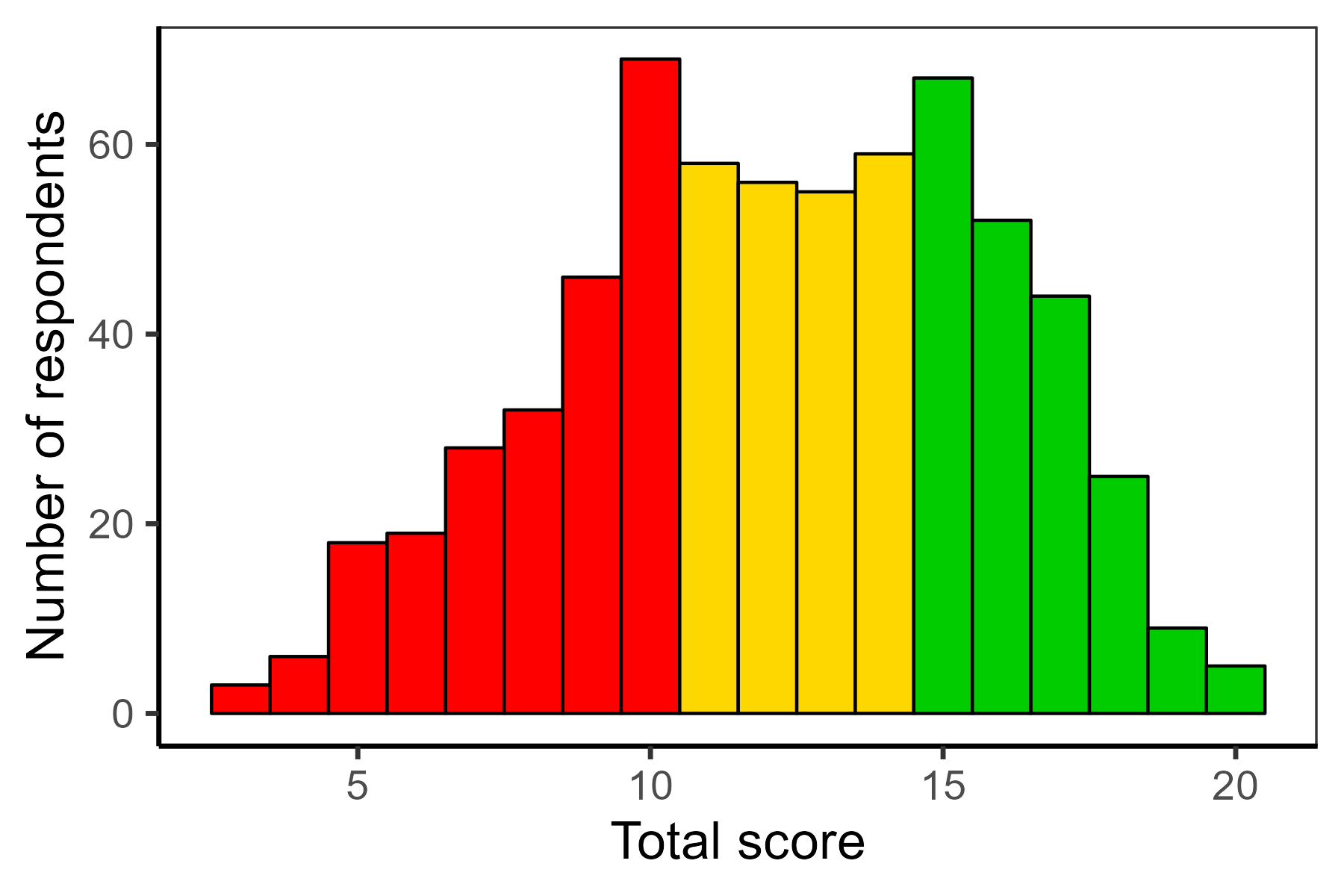
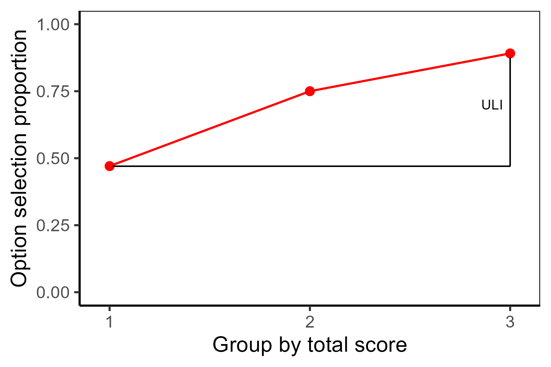
HCI dataset.
By a rule of thumb, ULI based upon thirds should not be lower than 0.2, except for very easy or very difficult items (Ebel, 1954). Items of medium difficulty with lower ULI are considered suspicious, and their content and wording should be checked.
ULI can be customized by determining the number of groups and by changing which groups are compared. This is especially helpful for admission tests where a certain proportion of students are admitted (Martinková et al., 2017). For example, if only one fifth of the students are admitted, the test developers may be interested in the discrimination calculated from the upper two fifths.
ULI typically depends upon the groups compared. ULI based upon the difference between the first and the last third will usually be lower than ULI based upon the first and the last fifth. Both of these will typically be higher than ULI based upon the fourth and the last fifth, except for difficult items.
Upper-lower index in the ShinyItemAnalysis package. We again consider the HCI dataset. Calculations of ULI are accessible with the gDiscrim() function of the ShinyItemAnalysis package. A default setting provides ULI based upon the difference in average item score between the first and the last third of the respondents, divided by the total test score.
gDiscrim(Data = HCI[, 1:20])
##  Item 1  Item 2  Item 3  Item 4  Item 5  Item 6  Item 7  Item 8  Item 9 Item 10
##  0.4580  0.3823  0.3832  0.3006  0.4633  0.4935  0.2440  0.4744  0.3439  0.3911
## Item 11 Item 12 Item 13 Item 14 Item 15 Item 16 Item 17 Item 18 Item 19 Item 20
##  0.3905  0.5162  0.5298  0.4962  0.4660  0.5972  0.1386  0.5209  0.5253  0.4596
Using the ULI, the lowest discrimination of 0.14 is estimated for item 17, while the highest discrimination of 0.53 is estimated for item 13.
Next, we compute ULI based upon the fourth and the last fifth of students. Argument k = 5 is used to specify a different number of groups, arguments l = 4 and u = 5 to set the lower and upper groups to be compared.
gDiscrim(Data = HCI[, 1:20], k = 5, l = 4, u = 5)
##  Item 1  Item 2  Item 3  Item 4  Item 5  Item 6  Item 7  Item 8  Item 9 Item 10
##  0.0783  0.0614  0.0085  0.2693  0.1778  0.1423  0.1942  0.1228  0.2889  0.1402
## Item 11 Item 12 Item 13 Item 14 Item 15 Item 16 Item 17 Item 18 Item 19 Item 20
##  0.0667  0.1434  0.1153  0.0265  0.1979  0.0778  0.2503  0.0180  0.0497  0.0836
For almost all items, ULI based upon three groups is larger than that based upon five groups comparing the two last fifths. This is not the case for item 17, for which the discrimination between the fourth and the last fifth was higher than discrimination between the first and the last third of respondents, which corresponds to a higher difficulty of this item, and suggests better discrimination between high ability students in this item.
Calculation of ULI is also implemented in the ItemAnalysis() function of the ShinyItemAnalysis package. The function can be used to jointly display all traditional discrimination indices, together with item difficulty and item SD (see Supplementary R code).
Item difficulty estimates together with selected discrimination indices (RIT, RIR, or generalized ULI), can be plotted jointly for all items using the so-called difficulty-discrimination plot provided by the DDplot() function of the ShinyItemAnalysis package. A discrimination index can be chosen by argument discrim. Additionally, when using discrim = "ULI", similar to the gDiscrim() function, one can further specify the number of groups k, and which upper group u and lower group l should be compared to calculate ULI. The DDplot() function offers the possibility to draw a user-specified threshold via the thr argument. In the example below, we provide a plot using the classical ULI calculation based upon three groups, with the default threshold of 0.2 (Figure 5.2 (a)), and using the threshold of 0.1 for ULI based upon the fourth and the last fifth for items in the HCI dataset (Figure 5.2 (b); see Supplementary R code for further plotting options).
DDplot(Data = HCI[, 1:20], discrim = "ULI")
DDplot(Data = HCI[, 1:20], discrim = "ULI", k = 5, l = 4, u = 5, thr = 0.1)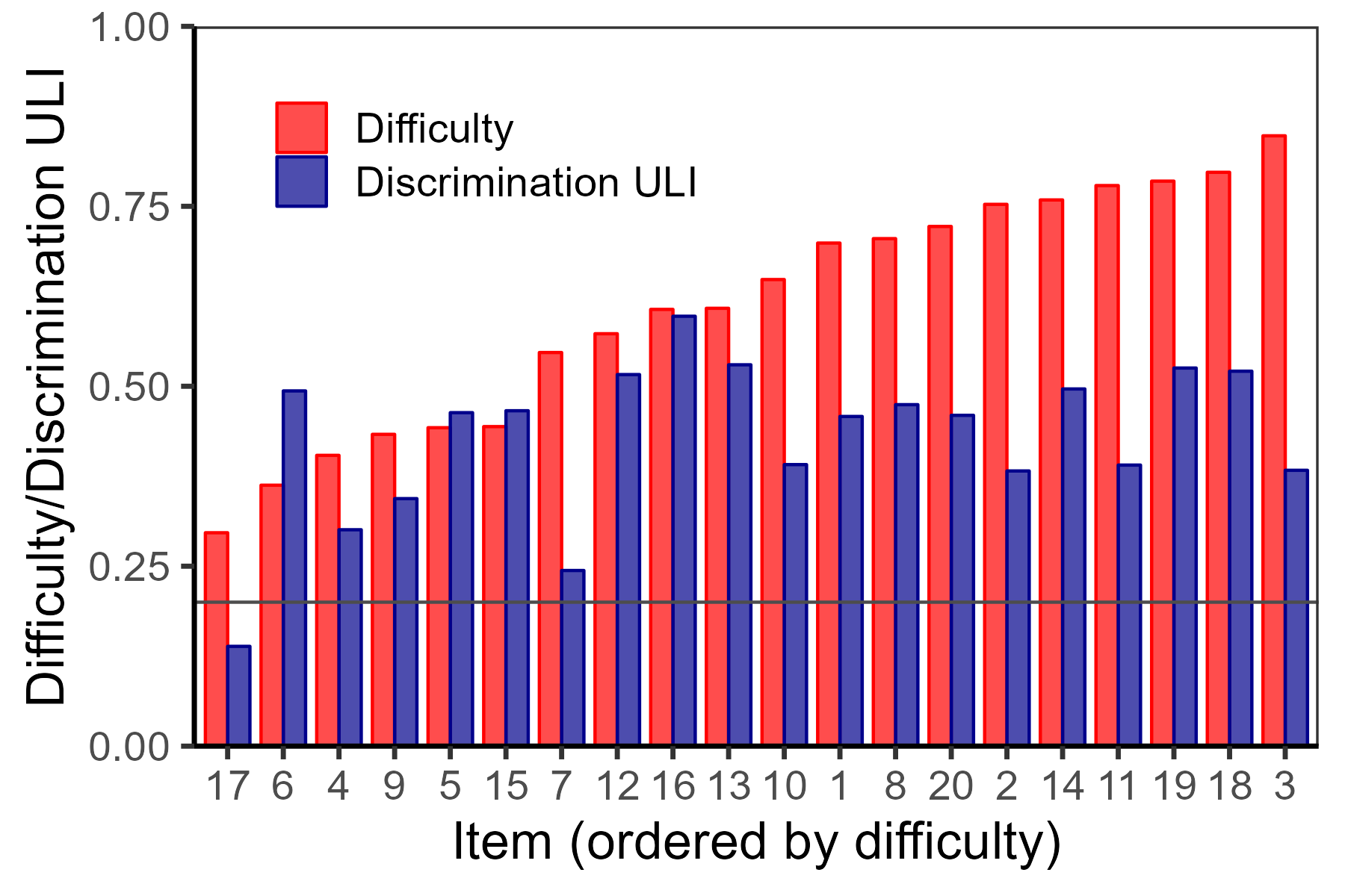
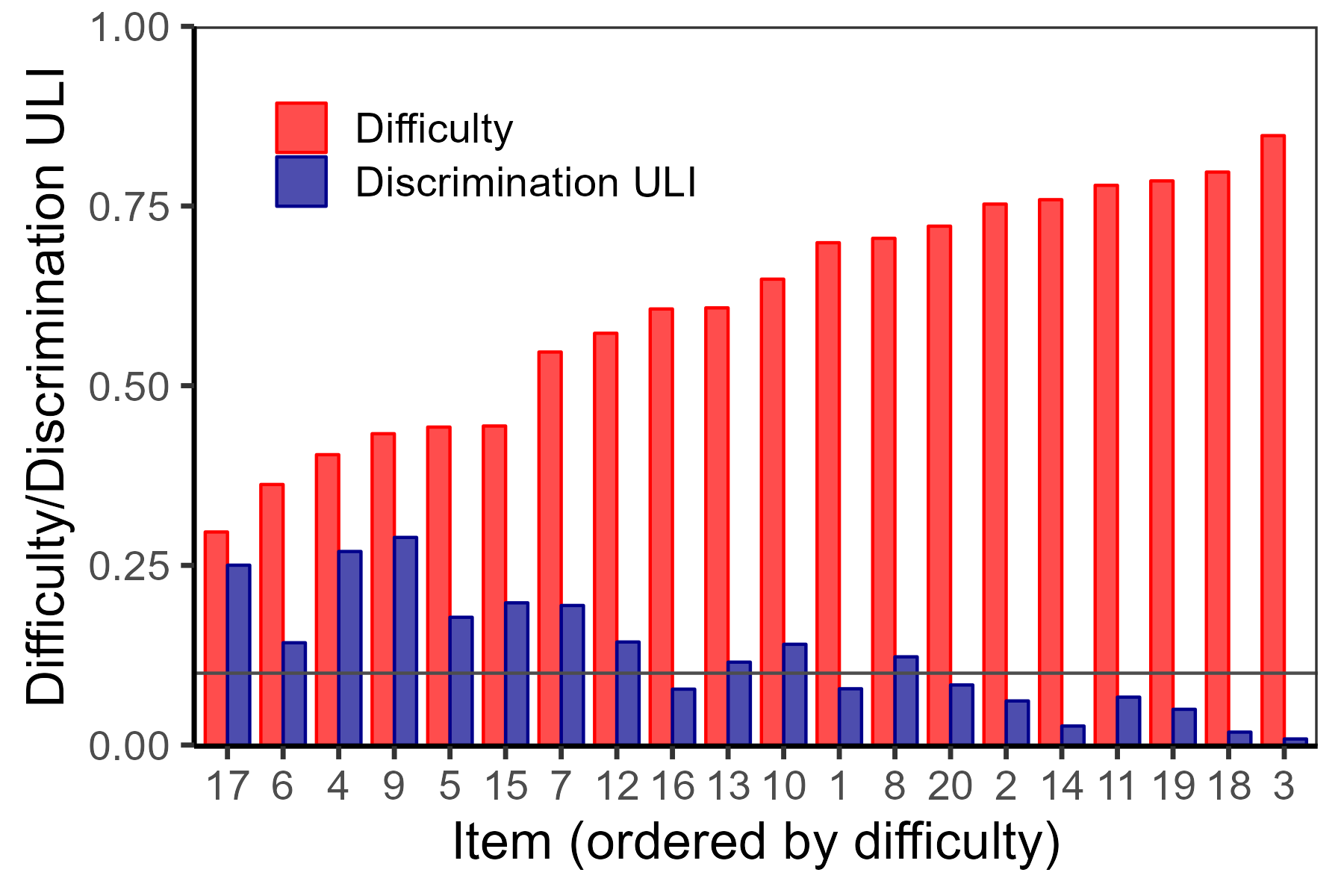
Figure 5.2 (a) suggests that item 17 should be further checked for content since its discrimination is below the threshold of 0.2, while Figure 5.2 (b) points out that item 17 is one of those that discriminates well between the highest ability students.
5.4 Item characteristic curve
To describe item functioning in more detail, the respondents may be divided into groups by their total score, and ratios of correct answers may be plotted out. The plotted curve is an estimation of item characteristic curve (ICC), which we will study closer in this and the next chapters. The ICC displays the relationship between the probability of answering an item correctly (on the \(y\)-axis) and the respondent’s level for the underlying trait which is being measured by the test (on the \(x\)-axis). In this chapter we consider the approximation of the latent trait by the total scores on the \(x\)-axis. Empirical ICCs of five hypothetical items are displayed in Figure 5.3.
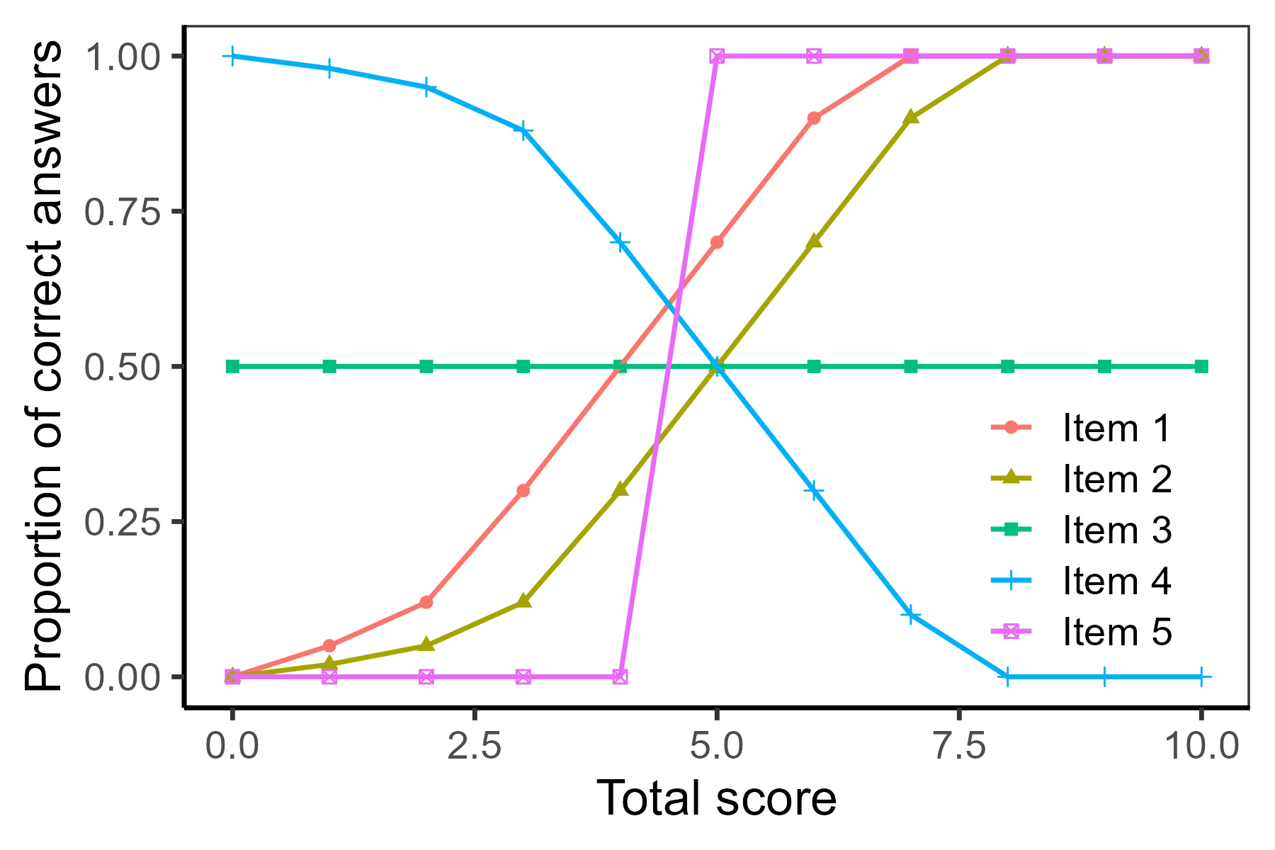
From the empirical ICCs, we can read the following information about item difficulty and item discrimination: The slope of the ICCs when \(y = 0.5\) may be used to estimate item discrimination, which is also applicable to ULI. An ICC of a well-discriminating item (see items 1, 2, and 5 in Figure 5.3) is increasing, i.e., has a positive slope; the respondents with a lower latent trait have a lower probability of answering an item correctly. A poorly discriminating item (see item 3) has a rather flat shape; the respondents with a lower latent trait have a similar probability of answering an item correctly when compared to respondents with a higher ability. These poorly functioning items should be checked for wording. A decreasing item (an item with negative slope, see item 4) signals that the item score is negatively related to the test score; the respondents with a higher total score, i.e., with higher levels of a latent trait, have a lower probability of answering the item correctly. Such items should also be checked for wording. When an item is inversely coded, it should be re-coded before an item analysis is performed. Finally, an item may be discriminating well at some levels of a latent trait but not discriminating well for other latent traits. As an example, item 5 is discriminating perfectly for respondents with a total score above 4 and below 5, but is not discriminating at all with respondents having a total score below 4, nor with respondents with total scores above 5. Note the trade-off between the slope and the range of total scores when an item is able to discriminate between the respondents.
Item difficulty may also be read from the ICCs. The definition is conceptually different from the traditional probability of correct items: We define here the item’s difficulty as attaining a total score which compares favorably to the total score needed to correctly answer the item with at least a 50% chance for success. In Figure 5.3 item 1 has a difficulty of 4, lower than the difficulty of 5 for item 2 and item 5.
Note that the estimated ratios get less precise with lower sample sizes. In such cases, the ratios are plotted usually only for 3, 4, or 5 groups, which are created based upon the total score, similar to the calculation for ULI.
5.5 Distractor analysis
In an educational context, multiple-choice items are commonly used. These consist of the question stem and several answer choices. Common types are single best answer, or odd one out, in which only one answer is correct or incorrect. Items with more than one correct option (multiple true-false items) are also sometimes used.
For multiple-choice items, difficulty and discrimination may be calculated for each response option. This allows us to evaluate the functioning not only of the correct option but also of so-called distractors. Distractors are incorrect response options included in a multiple-choice item to distract the respondent from the correct answer. The aim of the distractor analysis is to diagnose possible shortcomings (e.g., confusing wording) of the proposed response options in the test validation stage. It may also point to distractors which are either very rarely picked by the respondents or which are attracting well-performing respondents rather than the weaker ones, which are both undesirable. Finally, distractor analysis may also point to respondent misconceptions, and it may direct teaching after test administration.
To perform detailed distractor analysis, the ICCs of the correct option and the distractors may be plotted out. In the case of a lower number of respondents for some options, the respondents are usually divided into only 2, 3, 4, or 5 groups by their total score, similar to the calculation for ULI. Subsequently, a percentage of the respondents in each group who selected a given answer (correct answer or distractor) are calculated and displayed in a so-called distractor plot.
Distractor analysis in R. In R, the proportions of response options by a total-score group may be calculated using the DistractorAnalysis() function of the ShinyItemAnalysis package. We here use an unscored HCItest dataset and the HCIkey dataset which provides correct answers. We display distractor analysis for item 3 and item 17 using argument item, and we select the number of groups by using argument num.groups = 5.
data(HCIkey, HCItest, package = "ShinyItemAnalysis")
DistractorAnalysis(Data = HCItest[, 1:20], key = HCIkey, item = c(3, 17),
                   num.group = 5)
## $`Item 3`
## score.level
## response Group1 Group2 Group3 Group4 Group5
##        A     92    104    156    117     83
##        B     30     11      4      0      0
##        C     30     12     10      2      0
##
## $`Item 17`
## score.level
## response Group1 Group2 Group3 Group4 Group5
##        A     41     36     62     38     25
##        B     63     31     45     23     12
##        C     36     33     38     44     42
##        D     12     27     25     14      4
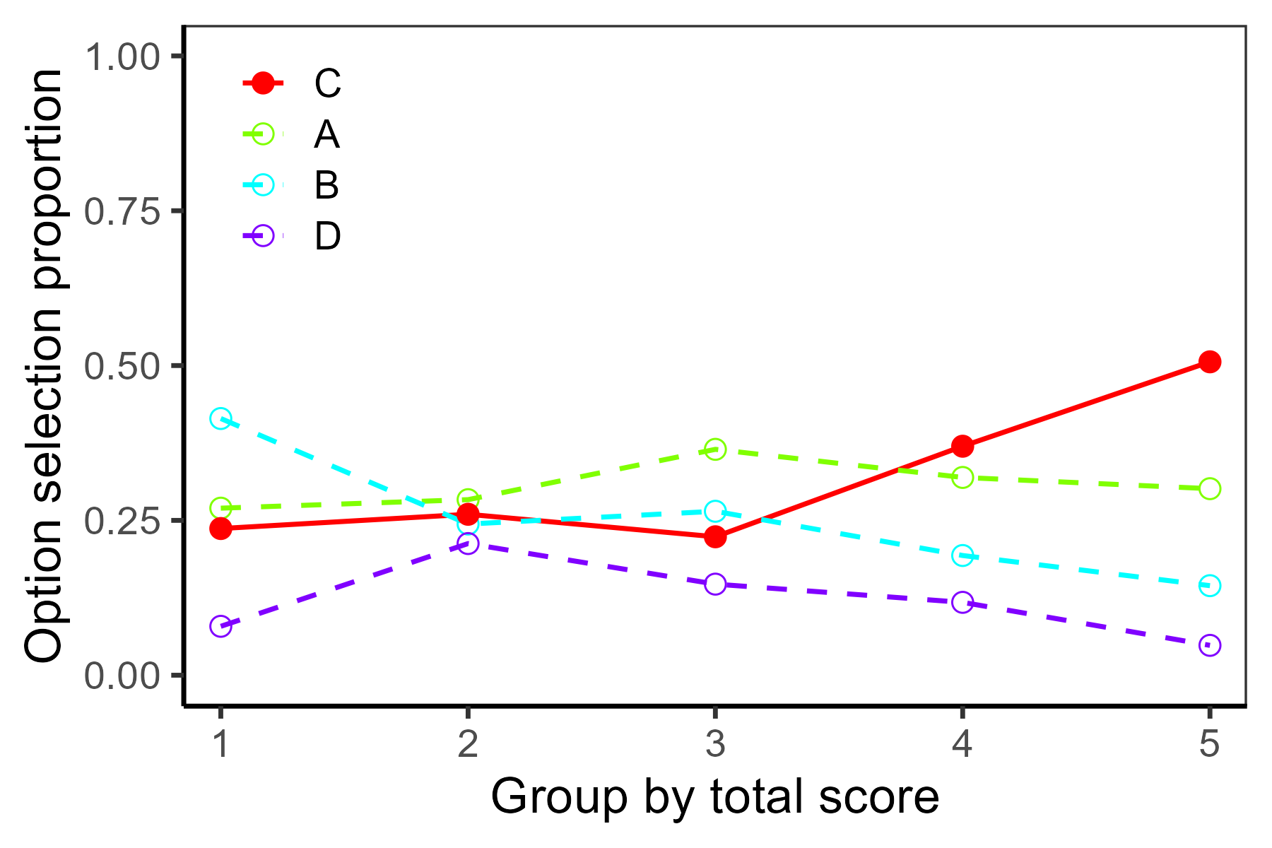
In item 3, the number of respondents who chose distractors decreases to 0 for higher ability groups, while this is not the case in item 17, where the distractor A was chosen by 25 respondents from the highest ability group, and distractors B and D were chosen by 12 and 4 respondents from this group.
Further, the plotDistractorAnalysis() function offers a graphical display of item functioning which may be used for the quick identification of well-functioning as well as suspicious items and response options.
plotDistractorAnalysis(Data = HCItest[, 1:20], key = HCIkey, item = c(3, 17),
                       num.group = 5, multiple.answers = TRUE)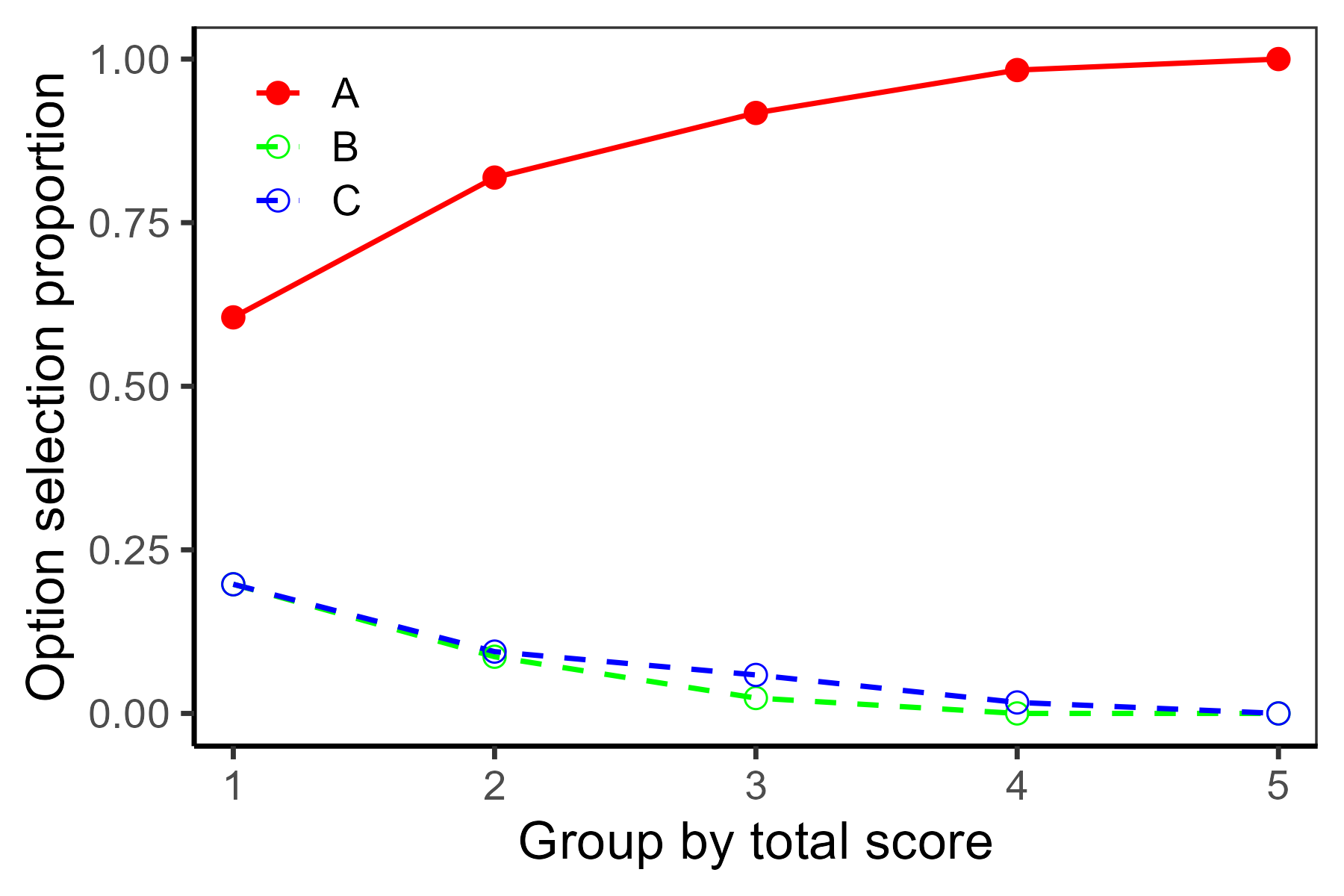
HCI dataset.
In a well-functioning item such as item 3 in the HCItest dataset, the correct answer is more often selected by high-ability respondents than by respondents with a lower total score; i.e., a solid line in the distractor plot is increasing with increasing ability (Figure 5.4 (a)). The distractors should work in an opposite direction, i.e., dotted lines should be decreasing. In the case of a suspicious item, such as item 17 in the HCItest dataset example, there may be no obvious differences between the functioning of the correct answer and the distractors (Figure 5.4 (b)). Closer inspection of item 17 may lead to a conclusion that the item functions well for the upper two fifths of the respondents, and the suspicious functioning for the lower three fifths of the respondents may be due to item difficulty.
5.6 Reliability if an item is dropped
In Chapter 4, Cronbach’s alpha Equation 4.13 was defined as an index describing internal consistency of the test. In the context of traditional item analysis, Cronbach’s alpha based upon all items except item \(i\), also denoted as alpha drop, can be used to detect inconsistent items:
\[ \alpha_i = \frac{m - 1}{m - 2} \left(1 - \frac{\sum_{j \neq i}\sigma^2_{Y_j}}{\text{Var}(\sum_{j \neq i} Y_j)}\right). \tag{5.9}\]
A sample estimate of Equation 5.9 is obtained by replacing the variances by their sample counterparts. Increase of Cronbach’s alpha \(\alpha_i\) after item removal signals an item inconsistent with the rest of the test.
Reliability if an item is dropped in the psych and ShinyItemAnalysis packages. In the HCI dataset example below, we employ the alpha() function from the psych package to calculate an estimate of Cronbach’s alpha Equation 4.13 of the original instrument and of Cronbach’s alpha after single items have been removed Equation 5.9.
psych::alpha(x = HCI[, 1:20])$total[1]
#  raw_alpha
#  0.7153
psych::alpha(x = HCI[, 1:20])$alpha.drop[, 1]
##  [1] 0.7042 0.7099 0.7007 0.7151 0.7054 0.6991 0.7220 0.7009 0.7114 0.7064
## [11] 0.7047 0.7016 0.6972 0.7001 0.7030 0.6952 0.7253 0.6943 0.6981 0.6997
The same result is reached with the ItemAnalysis() function of the ShinyItemAnalysis package in the Alpha.drop column.
ItemAnalysis(Data = HCI[, 1:20])$Alpha.drop
##  [1] 0.7042 0.7099 0.7007 0.7151 0.7054 0.6991 0.7220 0.7009 0.7114 0.7064
## [11] 0.7047 0.7016 0.6972 0.7001 0.7030 0.6952 0.7253 0.6943 0.6981 0.6997
Cronbach’s alpha of the original 20-item instrument is \(0.72\). Exclusion of most items leads to an expected lowering of the alpha estimate, while a slight increase can be observed after removal of items \(7\) and \(17\). This corresponds with their lower discrimination as measured by RIT, RIR, and ULI indices (see Section 5.3).
In practical applications, when Cronbach’s alpha of the scale without an item is higher than Cronbach’s alpha of the original scale, it might be tempting to consider permanent item removal. We, however, advice a caution. Removing such an item may lower instrument validity. Also, as was mentioned in Section 4.5, Cronbach’s alpha assumes unidimensionality of the scale; thus removing items based on increased alpha if item is dropped is unwise in instruments which are explicitly multidimensional.
5.7 Item validity
Item discrimination and distractor analysis may be performed with respect to a criterion variable other than the total score. If these item indices/analyses are calculated with respect to some criterion, such as student’s grade-point average or major, or patient’s health-status or score on a different assessment, they may be useful indicators of item criterion validity.
The relationship between item score \(Y_i\) and criterion variable \(Z\) can be described by their correlation \(\text{Cor}(Y_i, Z),\) and evaluated using the Pearson correlation coefficient Equation 2.13.
Item validity in R. In R, item validity may be calculated using the base cor() function within sapply() also specifying argument y. Alternatively, the ItemAnalysis() function of the ShinyItemAnalysis package may be used and correlations may be found under the Corr.criterion output.
ItemAnalysis(Data = HCI[, 1:20], criterion = HCI$major)$Corr.criterion
##  [1] 0.1173 0.1265 0.1541 0.0832 0.1274 0.0980 -0.0194 0.0949 0.0681 0.0968
## [11] 0.0782 0.0938 0.0909 0.0664 0.0859 0.0499  0.0312 0.1187 0.1295 0.0650
In the HCI dataset example, we see that item 3 correlates the best with the criterion describing a student’s planned major (Science vs. Other).
For all items, item correlation with a criterion may be displayed jointly with item difficulties in a difficulty-validity plot using the DDplot() function, see Figure 5.5 (a).
DDplot(Data = HCI[, 1:20], criterion = HCI$major, thr = NULL)To provide more detailed information about item functioning, distractor analysis may be performed, and the distractor plot may be plotted with respect to a criterion variable, using the plotDistractorAnalysis() function and its criterion argument. In the example below, we provide a distractor plot with respect to the binary variable major for item 5 of the HCI dataset. We specify the argument crit.discrete = TRUE to require a plot suitable for discrete criterion type.
plotDistractorAnalysis(Data = HCItest[, 1:20], key = HCIkey, item = 5,
                       criterion = HCI$major, crit.discrete = TRUE)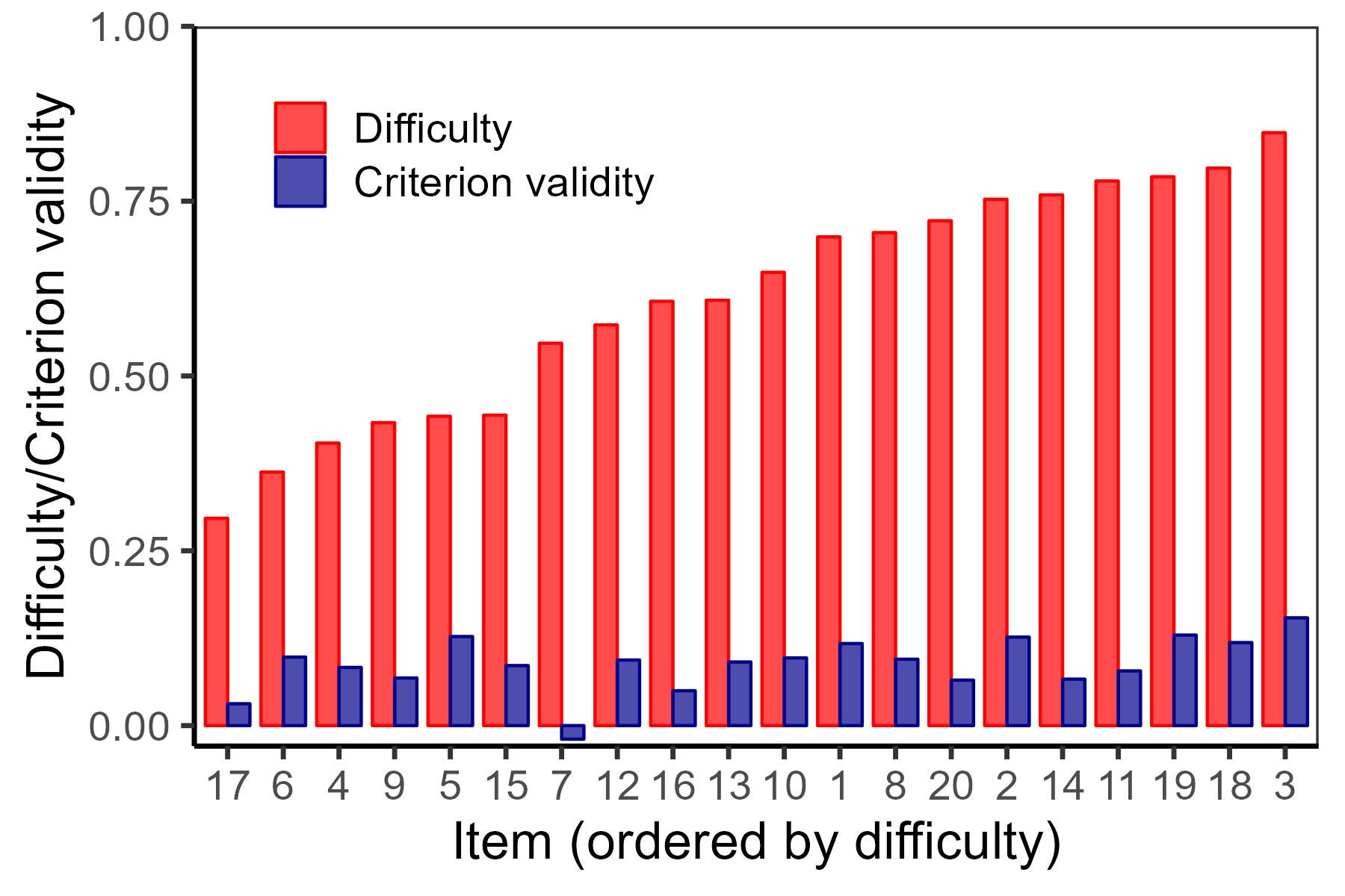
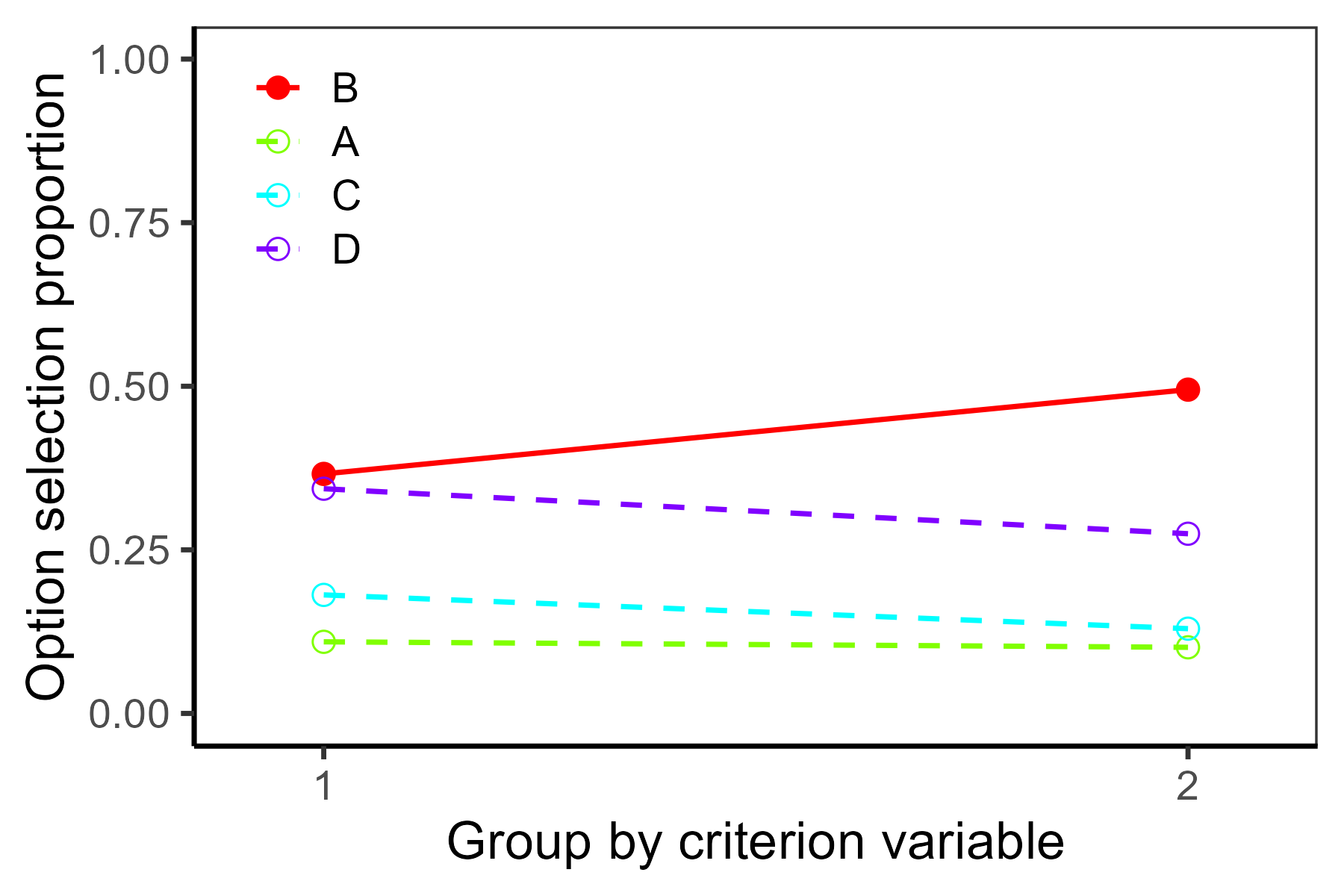
HCI dataset with respect to a planned major as a criterion variable.
Respondents studying Science as a major (group denoted as 2) tended to choose the correct answer of item 5 with higher probability (Figure 5.5 (b)).
5.8 Missed items
An important part of the traditional item analysis is a calculation of the percentage of cases when a given item was missed or not reached. A rule of thumb says that an item should be checked for content if 5 or more percent of the respondents missed it.
The percentage of non-reached, on the other hand, is calculated as a percentage of those who did not answer the item and any subsequent items in the test. Analysis of unreached items may be useful guidance about the length of the test or adequacy of time provided to answer the test.
Analysis of missed items in R. We demonstrate this analysis with the HeightInventory dataset.
We first display the number of missed answers in item 1 using the sum() and the is.na() functions. The number of respondents is obtained with the length() function. The percentage of missed answers is calculated simply as the percentage of those who did not answer the given item.
data("HeightInventory")
sum(is.na(HeightInventory[, 1]))
## [1] 9
length(HeightInventory[, 1])
## [1] 4885
100 * sum(is.na(HeightInventory[, 1])) / length(HeightInventory[, 1])
## [1] 0.1842
The first item was missed by 9 out of all 4885 respondents, which is 0.18%.
The sapply() function may be used to calculate the ratio of those who missed an item for all items. In the ItemAnalysis() function of the ShinyItemAnalysis package, this ratio is available in the Perc.miss column:
ItemAnalysis(Data = HeightInventory[, 1:26])$"Perc.miss"
##  [1] 0.1842 1.4125 0.6141 0.1024 0.1433 0.2047 0.0614 0.2047 0.1638 0.1433
## [11] 0.0614 0.0819 0.2252 1.5353 0.1842 0.1638 0.4504 0.0409 0.1228 0.1024
## [21] 0.1638 0.1638 0.1638 0.1433 0.0819 0.1228
The highest percentage of missed was in item 2: “I am taller than men of my age.” Closer inspection of the item shows that all respondents who skipped this item were females. However, the percentage of missing items is very low and may be neglected.
Next, we calculate the percentage of non-reached for each item. In the ItemAnalysis() function it is available under the Perc.nr column:
ItemAnalysis(Data = HeightInventory[, 1:26])$"Perc.nr"
##  [1] 0.0000 0.0000 0.0000 0.0000 0.0000 0.0000 0.0000 0.0000 0.0000 0.0000
## [11] 0.0000 0.0000 0.0000 0.0000 0.0000 0.0000 0.0000 0.0000 0.0000 0.0000
## [21] 0.0000 0.0000 0.0000 0.0000 0.0000 0.1228
The percentage of non-reached is zero for all items but the last one. In other words, all respondents who missed the last item at the same time answered the second to the last item. The ratio of non-reached for the last item is equal to the percentage of those who missed the item, 0.12%. This is a very small percentage, and it can be neglected.
5.9 Item analysis in interactive application
Interactive application ShinyItemAnalysis offers the traditional item analysis within the section Item analysis. On the very top of the Traditional item analysis tab, the difficulty-discrimination plot is offered to provide a quick overview of item functioning. The user may specify the difficulty index to be used (average scaled score vs. average score), and various discrimination indices including RIT Equation 5.6, RIR Equation 5.7, and generalized ULI Equation 5.8. When using generalized ULI, one can further select the number of groups or the upper and lower group to be compared. Finally, a difficulty-discrimination plot is supplemented by a threshold which can be used to identify suspicious items (Figure 5.6).
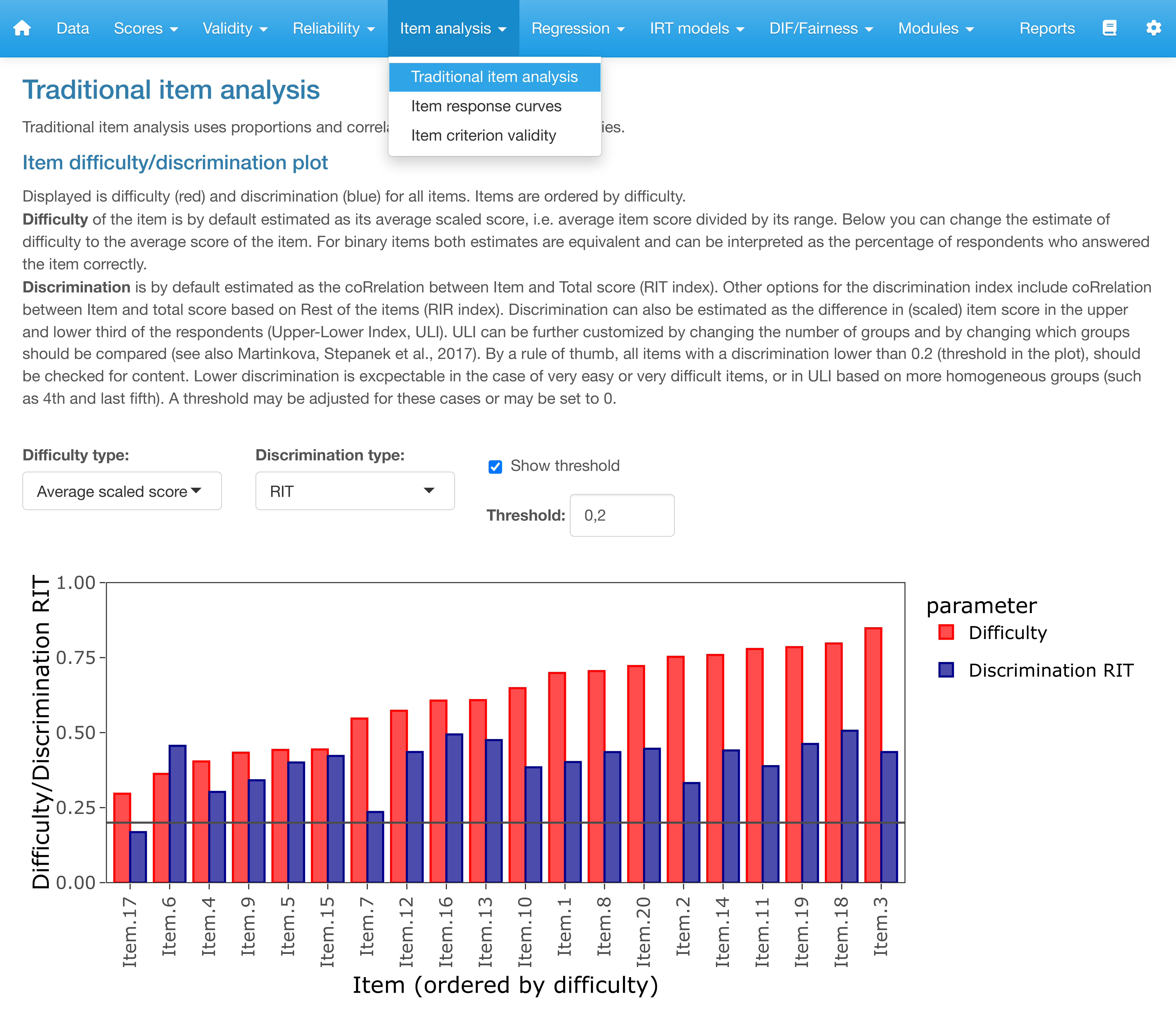
ShinyItemAnalysis interactive application for the HCI dataset.
Below the discrimination-distractor plot, the application provides a table with traditional item indices for each item. These include item difficulty, average item score, standard deviation, item discrimination as measured by ULI, RIT, or RIR. The table further provides Cronbach’s alpha calculated without an item (alpha drop) to assess reliability when item is deleted and to identify inconsistent items. If a criterion is provided, the table also offers item-criterion correlation to assess item validity. Finally, the ratio of students who missed or did not reach a given item is displayed.
Tab Item response curves offers more detailed analysis of individual items, including the distractor plots in the case of multiple-choice items, option selection ratios for a selected number of ability groups, and tables which provide these ratios as well as counts.
Finally, item analysis with respect to criterion is offered in the tab Item criterion validity. For this analysis, a criterion needs to be uploaded in section Data. A difficulty-validity plot shows items ordered by their difficulty, together with a criterion validity estimate. A distractor plot depicts item functioning with respect to a criterion in a more detailed way.
5.10 Summary
In this chapter, we have presented traditional item analysis, including characteristics of item difficulty, item discrimination, empirical ICC and distractor analysis. In connection with previous chapters, we have discussed reliability when item is deleted and we have defined item validity index. We have further discussed analysis of missing items. Implementations in the ShinyItemAnalysis package and interactive application were demonstrated.