1  Introduction

Measurement is present in many areas of our everyday life. In an educational context, these measurements include assessing academic achievement, certifying student qualifications and proficiency, high-stakes testing for school admission, as well as national and international large-scale assessment used to support policy decisions. In the area of psychology, measurements are used for assessing intelligence, personality traits, or attitudes. Health-related measurements include those of fatigue, depression, pain, quality of life, or well-being. Measurement is also present in other contexts, such as in hiring or promotion, peer review of articles, selection of grant proposals, and in numerous other areas.

What makes measurement in social sciences different from measuring height, weight, or blood pressure? The answer to this question is of key importance to understanding the specifics of the analytic and computational aspects involved. The main feature of measurement in social sciences is that it is typically not possible to directly measure the constructs of interest: The traits, such as math ability, leadership, level of depression, anxiety, or pain, are latent, which means unobservable, hidden. We have to use manifest variables, such as item responses on a questionnaire, to make inferences about these latent variables. Rather than a single manifest variable, we typically use a larger number of variables to measure the same latent construct, using multi-item measurement instruments. The measurement error is omnipresent and has to be enumerated and accounted for.

Psychometrics, as a field concerning psychological, educational, health-related, and other measurement in social sciences, is the disciplinary home for a number of statistical models and methods solving the challenges mentioned above. Psychometrics has contributed to many areas of statistics for many years, bringing not only motivation and inspiration but also providing computational improvements and solutions. A number of psychometric methods have been developed to draw inferences from empirical data and to gain quantitative proofs of measurement reliability, validity, or the functioning of single items. While closely related to statistical research, psychometrics has developed field-specific methods and terminology for models, tests, and indices.

1.1 Brief history of psychometrics

The year 1935, when the Psychometric Society was founded, may be considered an important milestone for psychometrics. However, the origins of psychometrics date much earlier and involve scientists from various fields. For an overview, see Jones & Thissen (2006), or the web page of the Psychometric Society. We mention at least a few of the important moments and figures below.

Carl Friedrich Gauss (1777–1855), a German mathematician and physicist, studied measurement errors in the context of astronomy and orbital prediction. He employed the method of least squares and a statistical distribution which is now known as the Gaussian or normal distribution. In the context of recording the transition time of stars, another German astronomer, Friedrich Bessel (1784–1846), who corresponded regularly with Gauss, noticed that when several observers are employed simultaneously, they determine slightly different values. He further elaborated this concept into a “personal equation” enabling an estimation and correction for rater biases employing the method of least squares. As a result, the measurement error and reaction times became a major topic in experimental psychology of the time.

Sir Francis Galton (1822–1911), a British scientist known for achievements in many scientific areas, is also often referred to as “the father of psychometrics”. Influenced by Charles Darwin, he employed statistical methods to study human differences and inheritance on data measured in his Anthropometric Laboratory in London. He noticed that above-average height fathers tended to have sons shorter than themselves, while shorter fathers tended to have sons taller than themselves, a concept he termed “regression towards mediocrity”. This phenomenon, now termed as “regression towards the mean” is present in many fields including psychological, educational, and health-related measurement. While Galton mainly studied linear relationships, and correlation and prediction, his initial input later gave a start to a wide range of regression models. His numerous papers and books include the Brain journal paper, “Psychometric Experiments”, in which he describes psychometrics as the “art of imposing measurement and number upon operations of the mind” (Galton, 1879).

The British psychologist Charles Edward Spearman (1863–-1945), influenced by Galton, worked on a general intelligence factor which he termed g factor. It should be noted that Spearman was a University College colleague of Karl Pearson (1857–-1936), who is credited with establishing the discipline of statistics. While Spearman’s main focus lay in experimental psychology, he was also well known for his work in statistics: Spearman’s rank correlation coefficient — a nonparametric version of Pearson’s correlation coefficient, for articles on correction for attenuation, and for initial development of factor analysis.

In France, Alfred Binet and Théodore Simon developed the Binet-Simon IQ test, with the aim of measuring higher cognitive abilities, and to identify students who did not learn effectively from regular classroom instruction. In 1905, they introduced the concept of mental age. English translations of the test followed, notably by Lewis M. Terman in 1916, who defined the IQ score as a quotient of mental age divided by chronological age multiplied by 100.

During World War I, psychological examination of U.S. Army recruits was of interest. A statistical unit working on development of Army Alpha and Beta test batteries involved Edward Lee Thorndike, Arthur S. Otis, and Louis Leon Thurstone, the future first president of the Psychometric Society. Initial meetings of the founding fathers of the society concerned creation of a new journal for publication of psychometric research. The first issue of the journal Psychometrika followed shortly after, in 1936.

During World War II, the Army General Classification test was developed, and psychometric research was concentrated on this test to assure its quality. Influenced by the work on army test batteries, the Stanford Achievement Test was delivered to measure student learning at school. Development of further educational tests followed. The Educational Testing Service (ETS) was founded in 1947, which produced the Scholastic Aptitude Test (SAT). Numerous psychological, educational, health-related, and other measurement instruments have been developed and established since those times.

1.2 Measurement in social sciences

The process of measurement in social sciences includes a number of steps. As a general principle, before considering any psychometric analysis, the data and measurement quality needs to be assured by the process of measurement development. The general guidelines for test development are provided in the Standards for Educational and Psychological Testing by the American Educational Research Association (AERA), the American Psychological Association (APA), and the National Council on Measurement in Education (NCME) (2014). As test development itself is not the focus of this book, we will only mention briefly the main important steps. For more details, the reader is referred to the Handbook of Test Development by Lane et al. (2015).

Defining the construct of interest is perhaps the most important part of measurement development. Without a very clear and precise idea about what is intended to be measured, the measurement scores will seldom be valid. Naming and defining the domain to be measured are followed by developing content specifications to guide item development. In the context of educational measurement, this step includes creating conceptual frameworks, or what is sometimes called blueprinting, i.e., the precise and detailed description of the foundation stones from which the measurement instrument should be composed.

Item development is the key component in multi-item measurement. Suitable item formats need to be selected and the items need to be written in such a way that they align with the construct and its components. High quality items are those which are reviewed by a number of reviewers for their quality and pretested on a sample of respondents from the specific interest group.

Rater training is important when a number of different raters are used to perform the measurement. This includes providing clear and detailed direction about what is to be rated and how it is to be rated, a detailed rubric. Rater training may be complemented by an assessment of the alignment of their ratings compared to a pre-specified gold standard, and formalized by a rater certification.

Once the measurement data are collected, the psychometric analyses, which are the main focus of this book, may take place. These analyses may provide empirical proofs for complex validation of the instrument, or assign scores to the respondents or ratees, but can also provide other useful evidence. We describe the validation process and the process of respondent scaling briefly here, while the later chapters of this book will provide more detailed information on psychometric tools for each single step, especially focusing on the computational aspects.

Collecting proofs of test validity. While an important part of validity evidence stems from the instrument development process, a number of different psychometric analyses may be performed to provide empirical evidence of instrument validity, i.e., to provide proofs that the instrument measures what it is intended to measure. These analyses include evidence based on external criteria, such as correlations with scores from other instruments. Other psychometric analyses can focus on between-item correlations and the internal structure of the test. See Chapter 2 and Chapter 3 for details on collecting proofs of test validity.

Collecting proofs of test reliability. Assessing measurement reliability is especially important, as this reliability is what limits the measurement validity. Is the measurement consistent when repeated in time, by different raters or on different occasions? How much error is due to external sources or due to random noise? Chapter 4 provides further details on analyses relevant for collecting proofs of test reliability.

Analyzing item functioning. The measurement instrument is typically composed of several items, and to address the quality of the entire instrument, it is imperative to take a look at these individual items. Do all items work properly and discriminate well between respondents? Is guessing an issue? How much information does an individual item carry for respondents of a certain ability level? We provide traditional item analysis in Chapter 5, we start building regression models for item description in Section 9.4, and we describe the Item Response Theory (IRT) models in Chapter 7 and Chapter 8.

Analyzing impact of group membership and other covariates. In order to ensure instrument fairness but also to understand strengths as well as weaknesses and misconceptions of different groups of respondents, the test and item functioning needs to be analyzed with respect to groups and other respondent or rater characteristics. This is especially important when considering that, oftentimes, only a relatively small selection of items is presented to the respondent, or a selection of raters is used to rate a subject or object of measurement. We focus on group effects in Chapter 9, while we also discuss covariates such as grouping variables in preceding chapters.

Selecting optimal items. In the case of larger item banks, only a portion of the items is offered at a time to the respondent. Detailed information on item functioning can then be used to design optimal selection of items in an adaptive setting. In other situations, when a number of test versions is used, information about item properties is being used to equate resulting ability estimates or to link the test versions. We discuss adaptive tests in Chapter 10.

Scaling. Eventually, the measurement instrument is used to assign scores to respondents or other rated subjects/objects. We discuss traditional scaling methods in Chapter 1, factor analytic approach in Chapter 3, and methods based on IRT models in Chapter 7 and Chapter 8.

While the general concepts are common among all areas of multi-item measurement or ratings from multiple raters, different fields have their specifics in the psychometric methods needed for measurement. We will now turn to a discussion of these specifics.

1.2.1 Educational measurement

An educational measurement typically aims at assessing knowledge, ability, or academic achievement. The status of this field, including many aspects of psychometrics, is summarized in the latest edition of the Educational Measurement (4th Edition) edited by Brennan (2006). In most cases the assessment instrument is developed to measure a one-dimensional construct, such as knowledge of a certain subject or concept.

Educational assessment may have a number of purposes, which may in turn affect the psychometric analyses used on data from these assessments. For example, formative tests are used throughout the course to aid learning. In contrast, summative assessment is typically used at the end of the course to assign students a grade.

Various testing situations further differ in the stakes that are involved: So called high-stakes tests have major consequences, such as awarding a high school diploma based upon the exit/matura examination, or entering a university based upon an admission test. Contrarily, the low-stakes tests include the classroom, national, or international testing used for monitoring student progress.

The criterion-referenced tests compare the score with a predefined cut score or other criterion. In this type of test, the performance of other respondents does not affect the respondent, as is the case on a driving test. The norm-referenced tests, on the contrary, compare the respondent score with the score of other respondents. The final score in this type of tests provides the information about the percentage of the population of given characteristics (age group, etc.) which has a higher, or a lower score.

Testing situations also differ by other aspects, such as the sample size, i.e., the number of students taking the test. This may greatly influence the psychometric analyses available for the given sample size. For example, some of the IRT models presented in Chapter 7 cannot be fitted for small sample sizes, and their use on data from classroom testing may not be possible.

Conceptual tests are knowledge assessments focusing on a certain knowledge area or a concept. As an example, McFarland et al. (2017) described the development and validation of the Homeostasis Concept Inventory (HCI), a conceptual test assessing an undergraduate level of understanding of the concept of homeostasis, the way the body regulates physiological systems. The authors performed a thorough validation study including a number of psychometric analyses of the responses of a high number of undergraduate students on the test. We use the HCI dataset throughout the book for demonstration purposes.

Language tests such as the Test of English as a Foreign Language (TOEFL)1 are specific in that they analyze respondent speaking and writing abilities. The Duolingo English Test2 may be taken any time. Principles of adaptive testing and text analysis with machine learning are used to automatically generate test items and to score test-taker item responses.

State matura examinations are high-stake tests organized in many countries as high school exit examinations. In some countries, these tests are further used for university admissions; the typical example is Great Britain’s A-levels. In this book, we use data from the Czech Republic matura examination to demonstrate some of the psychometric analyses.

Admission tests to universities and high schools are yet another area of educational assessment which are of great importance. The entrance exams may be a more general form of aptitude tests such as the SAT3, or a more focused admission test, such as the Medical College Admission Test (MCAT)4, Graduate Medical School Admission Test (GAMSAT)5, Graduate Management Admission Test (GMAT)6, and others. With a high number of students and specific times when the exam may be taken, one of the key aspects is ensuring that the scores from different test dates are comparable.

National/state testing is implemented in many countries to provide information on school quality or for diagnostic purposes, such as early detection of failing students. In the United States, the “No Child Left Behind” act led to implementation of yearly state testing across the country. State testing exists in most countries, although many test only those students from the final grades of given educational stages. In Europe, the state testing is typically low-stakes both for the students and for the schools. In some countries it is possible to link individual data from different years and perform a longitudinal analysis. Some practical examples will be demonstrated on the data from the Czech Longitudinal Study in Education (CLoSE), which administered tests in mathematics, reading, Czech language, and learning competence to the same students in Grades 4, 6, and 9 (Greger et al., 2022).

International large-scale assessment, abbreviated as ILSA7, is used for international educational policy development. The studies include the Programme for International Student Assessment (PISA), Trends in International Mathematics and Science Study (TIMSS), or Progress in International Reading Literacy Study (PIRLS). Large international teams of experts are present during test development, the tests and analytic approaches are typically very well documented, and a great deal of data is publicly available.

1.2.2 Psychological assessment

While educational measurements are typically unidimensional, the assessment instruments in psychology are very often multidimensional. For example, the big five model, also known as the five-factor model, is probably the most widely accepted personality theory model. It states that personality can be boiled down to five core factors, known by the acronym CANOE or OCEAN: Openness, Conscientiousness, Extroversion, Agreeableness, and Neuroticism. Inventories used to measure these five factors of personality include the Big Five Inventory (BFI) and its revised version BFI-2 (Soto & John, 2017). As an example, we use the BFI2 dataset from the Czech adaptation of the revised version (Hřebı́čková et al., 2020).

Psychological tests are typically norm-referenced, and development of population norms is usually an important part of test development. Contrary to educational testing, the psychological testing typically uses ordinal scales such as the Likert scales, “strongly agree” – “agree” – “neutral” – “disagree” – “strongly disagree”. Unlike in educational testing, there are usually no correct or wrong answers to an item.

Psychological measurement also assesses cognitive functions (e.g., memory or intelligence), emotional states, attitudes, and often the diagnosis of psychological disorders is of interest. More information on psychological measurement can be found in Goldstein et al. (2019) or in Thorndike & Thorndike-Christ (2010).

1.2.4 Other areas of measurement

Measurement of latent traits with multi-item instruments or multiple raters is also present in other areas. In organizational research, raters are typically involved in hiring of new employees (Martinková et al., 2018). The validation of such hiring instruments and procedures involves gaining empirical evidence of their predictive power: To what extent is the rater able to predict the future value of the teacher to their students? In addition, inter-rater reliability is of interest as a way to assess the consistency of the raters. Functioning of the individual criteria being rated may provide information on possible further improvements of the instrument.

As an example of another area, in grant proposal selection, peer review is an important part of the process. Raters and committees are involved in selection of the top grant proposals to be funded. In this book, we make use of peer review data from the American Institute of Biological Sciences (AIBS) (Erosheva et al., 2021) to demonstrate aspects of the inter-rater reliability analysis. Other areas of measurement include journal article peer review, and customer satisfaction surveys.

1.3 Measurement data in this book

The datasets used in this book cover all above-mentioned areas of measurement in social sciences. The datasets are available in the ShinyItemAnalysis package and also on the book web page.

AIBS Grant Peer Review Scoring. The AIBS Grant Peer Review Scoring dataset (Erosheva et al., 2021) comes from a scientific peer review of biomedical applications from a collaborative biomedical research funding program of the AIBS (2014–2018). Three assigned individual reviewers were asked to provide scores and commentary for the following application criteria: Innovation, Approach/Feasibility, Investigator, and Significance (Impact was added as a scored criteria in 2014). Each of these criteria is scored on a scale from 1.0 (best) to 5.0 (worst) with a 0.1 gradation, as well as an overall score. The dataset further contains information on the review year, proposal anonymized ID and type, investigator’s anonymized ID, organization type, gender, rank, and degree, as well as each reviewer’s anonymized ID, institution type, gender, rank, and degree.

Anxiety. Anxiety is a real dataset originally from the lordif package. It contains responses from 766 respondents sampled from a general population to the PROMIS anxiety scale composed of 29 Likert-type questions with a common rating scale. Besides item responses, this dataset also contains the age, gender, and education category as further characteristics of respondents.

The Next Big Five Inventory (BFI2). The BFI2 dataset (Hřebı́čková et al., 2020) consists of responses by 1,733 Czech respondents (730 males, 1,003 females) to the Next Big Five Inventory BFI-2 (Soto & John, 2017) measuring personality in five domains: Extroversion, agreeableness, openness, conscientiousness, and neuroticism. It contains responses to 60 ordinal items from each respondent. Besides item responses, the dataset contains the age, education, and gender membership for each respondent.

Czech matura. The CZmaturaS dataset comes from the Czech matura exam in mathematics. The matura exam was assigned in spring 2019 to students from Grade 13, at the end of their secondary education. The dataset consists of responses from a random sample of 2,000 out of 15,702 students. It includes 75 variables including item answers, scored items, the school type, and a binary variable on whether this was the first attempt at the matura exam, or if it was a repeated exam. The ShinyItemAnalysis package also includes the CZmatura dataset, which contains data from the complete set of 15,702 students.

Eysenck Personality Inventory – Impulsivity Subscale (EPI-A). The EPIA (Ferrando, 2002) is a real dataset originally available in the EstCRM package (Zopluoglu, 2015). The data capture the responses of 1,033 undergraduates to five items from the Spanish version of the EPI-A impulsivity subscale. Their responses were checks on a 112 mm line segment with two end points: almost never and almost always. The item score was defined as the distance in mm of the check mark from the left end point (Ferrando, 2002).

Graduate Management Admission Test (GMAT). The GMAT is a simulated dataset originally available in the difNLR package. The dataset represents the responses of 2,000 subjects (1,000 males, 1,000 females) for a multiple-choice test of 20 items. The answers were generated using item parameters of the real GMAT exam (Kingston et al., 1985). The distribution of total scores was the same for both groups; however, the first two items were manipulated to function differently for the two groups (Martinková, Drabinová, et al., 2017). The GMAT dataset also contains a simulated continuous criterion variable.

Homeostasis Concept Inventory (HCI). The HCI (McFarland et al., 2017) is a 20-item multiple-choice instrument that assesses how well undergraduates understand the critical physiological concept of homeostasis. The HCI was validated on a main sample of 669 undergraduate students and smaller samples of 45, 16, and 10 students. Several datasets from the original study are available in the ShinyItemAnalysis package and presented in this book:

  • The HCIdata contains the answers from the main sample of 669 undergraduates to multiple-choice items of the HCI test (variables A1–A20), the scored items (variables QR1–QR20), the total score (total), and number of contextual variables: gender, major, year of study, minority membership, and other.
  • The HCItest contains answers and the HCI dataset contains scored items of a subsample of 651 undergraduate students (405 males, 246 females) who disclosed their gender.
  • The HCIkey is a nominal vector with 20 values representing correct answers to items of the HCIdata and HCItest dataset.
  • The HCIlong dataset contains the HCI data in the long format (see Section A.4.3).
  • The HCIgrads dataset consists of the responses of 10 graduate students.
  • The HCItestretest dataset consists of the responses of 45 students to HCI from two occasions (test and retest), who took no courses on homeostasis between the two occasions.
  • The HCIprepost dataset contains the pretest and posttest score of 16 students who received instruction on homeostasis within a physiology course between the two test occasions.

Height Inventory. The HeightInventory dataset consists of the responses of 4,885 Czech respondents (1,479 males, 3,406 females) to a Height Inventory (Rečka & Cígler, 2020). The Height Inventory contains 26 ordinal items of self-perceived height, such as “A lot of trousers are too short for me” or “In a crowd of people, I still have a comfortable view”, rated on a scale 1 – strongly disagree, 2 – disagree, 3 – agree, 4 – strongly agree. The dataset further contains self-reported height (in centimeters) and gender membership of each respondent.

Learning to Learn (LtL). The LearningToLearn (Martinková et al., 2020) is a real longitudinal dataset from CLoSE study (Greger et al., 2022). Among other variables, it primarily contains the binary-scored responses of 782 secondary-school students to a (mostly) multiple-choice test consisting of 41 items within 7 subscales of the test of learning competencies. Item responses from Grade 6 and Grade 9 are available for each respondent. The school track (variable track_01 or track) is available, with 391 students attending a basic school and 391 pursuing selective academic school. The LearningToLearn dataset was created from a larger sample of respondents using a matching algorithm to achieve similar characteristics for both tracks in Grade 6.

Medical School Admission Test. Several real datasets of an admission test to medical school (Martinková, Štěpánek, et al., 2017) are presented in this book:

  • The dataMedical contains binary-scored items of an admission test to medical school for 2,392 applicants.
  • The dataMedicalgraded is an ordinal version of the dataMedical dataset. Each item was graded from 0 to 4 points. A maximum of 4 points was given if all of the correct answers and none of the incorrect answers were selected. Similarly to the dataMedical dataset, this ordinal dataset also includes the gender variable and study status as the criterion variable.
  • The MSATB dataset is a subset of a real medical school admission test for Biology from the difNLR package (Drabinová & Martinková, 2017; Hladká & Martinková, 2020). This dataset represents responses of 1,407 subjects (484 males, 923 females) for a selection of 20 multiple-choice items. The first item was previously detected as functioning differently for the two genders.

Test Anxiety. The TestAnxietyCor dataset contains between-item correlations for 20 items of the Test Anxiety inventory. The items cover both the psychological aspects of test anxiety, e.g., thinking about grades, thinking about getting through school, as well as physiological reactions of the nervous system, e.g., uneasy, upset feeling, freeze up, etc. See Bartholomew et al. (2008) for more details.

1.4 Psychometrics with R

A number of software packages are available for psychometric analysis, many of which contain commercial software for specific purposes. The IRT models are offered with IRTPRO (Paek & Han, 2013), flexMIRT (Chung & Houts, 2020), Winsteps (Linacre, 2021), or ConQuest (Adams et al., 2020). The factor analytic approach, path analysis, and more generally the structural equations models are available with LISREL (Jöreskog & Sörbom, 1996), EQS (Bentler, 2006), Amos (Arbuckle, 2011), Mplus (Muthén & Muthén, 2017), or gllamm which is implemented in Stata (Rabe-Hesketh et al., 2004).

In this book, we use R (R Core Team, 2022) which is a freely available statistical environment. There are a number of things that make R a great choice for psychometric analysis: Besides being free, it is also open source software, meaning that the code is available for the user, and it is possible to check what a given function does or how the methods are implemented. It offers up-to-date methods as a number of statisticians and researchers from different fields implement the newly published algorithms and methods in R. There is a huge community around R; thus finding an answer to a question is not a hard task. R also offers excellent graphical instruments.

The basic functionality of the language R is enhanced by numerous packages authored by R contributors. Many R packages have been developed to cover general psychometric concepts as well as specific psychometric topics. For an overview, see the subject specific CRAN Task View. In addition, some of the psychometric models can be implemented by using general packages such as lme4. A brief description of the packages used in this book including full citation, the title of the package, and chapters in which the package is used is provided in the table below.

R package Version (Year) Citation Title Chapters
aod 1.3.2 (2012) Lesnoff & Lancelot (2012) Analysis of Overdispersed Data 9
brms 2.19.0 (2023) Bürkner (2017) Bayesian Regression Models using ‘Stan’ 4, 7
catR 3.17 (2022) Magis & Raîche (2012) Generation of IRT Response Patterns under CAT 10
deltaPlotR 1.6 (2018) Magis & Facon (2014) DIF using Angoff’s Delta Plot Method 9
DFIT 1.1 (2021) Cervantes (2017) Differential Functioning of Items and Tests 9
difNLR 1.4.2 (2023) Hladká & Martinková (2020) DIF and DDF Detection by Non-Linear Regression 9
difR 5.1 (2020) Magis et al. (2010) Collection of Methods to Detect DIF 9
equateIRT 2.3.0 (2022) Battauz (2015) IRT Equating Methods 9
eRm 1.0.2 (2021) Mair et al. (2020) Extended Rasch Modeling 7, 8
ggdendro 0.1.23 (2022) de Vries & Ripley (2020) Create Dendrograms Using ‘ggplot2’ 3
ggplot2 3.4.1 (2023) Wickham (2016) Elegant Data Visualisations 1–10
GPArotation 2022.10.2 Bernaards & Jennrich (2005) GPA Factor Rotation 3
gtheory 0.1.2 (2016) Moore (2016) Apply Generalizability Theory with R 4
hemp 0.1.0 (2023) Bulut (2020) Handbook of Educational Measurement Companion 4
lattice 0.20.45 (2021) Sarkar (2008) Trellis Graphics for R A
lavaan 0.6.15 (2023) Rosseel (2012) Latent Variable Analysis 3
lme4 1.1.32 (2023) Bates et al. (2015) Linear Mixed-Effects Models 4, 7
lmtest 0.9-40 (2022) Zeileis & Hothorn (2002) Testing Linear Regression Models 2
lordif 0.3.3 (2016) Choi et al. (2011) Logistic Ordinal Regression DIF 9
ltm 1.2.0 (2022) Rizopoulos (2006) Latent Trait Models under IRT 7, 8
mirt 1.38.1 (2023) Chalmers (2012) Multidimensional Item Response Theory 1, 7–10
mirtCAT 1.12.2 (2022) Chalmers (2016) Computerized Adaptive Testing with mirt 10
moments 0.14.1 (2015) Komsta & Novomestky (2015) Moments, Cumulants, Skewness, Kurtosis 1
msm 1.7 (2022) Jackson (2011) Multi-State Markov and Hidden Markov Models 6, 9
nlme 3.1.162 (2023) Pinheiro et al. (2020) Linear and Nonlinear Mixed Effects Models 6
nnet 7.3.18 (2022) Venables & Ripley (2002) Feed-Forward Neural Networks 1–5, 7
psych 2.3.3 (2023) Revelle (2020) Psychological, Psychometric Research 4
psychometric 2.3 (2022) Fletcher (2010) Applied Psychometric Theory 4
remotes 2.4.2 (2021) Hester et al. (2021) R Package Installation from Remote Repos A
semPlot 1.1.6 (2022) Epskamp (2019) Path Diagrams and Visual Analysis of SEM 3
shiny 1.7.3 (2022) Chang et al. (2021) Web Application Framework for R A
ShinyItemAnalysis 1.5.0 (2023) Martinková & Drabinová (2018) Test and Item Analysis via Shiny 1–10
SIAmodules 0.1.0 (2023) Martinková & Netík (2023) Modules for ‘ShinyItemAnalysis’ 4, 10
TAM 4.1.4 (2022) Robitzsch et al. (2021) Test Analysis Modules 7
tidyverse 2.0.0 (2023) Wickham et al. (2019) Easily Install and Load the ‘Tidyverse’ A
VGAM 1.1.8 (2023) Yee (2015) Vector Generalized Linear and Additive Models 6

In Appendix A (see also Supplementary R code), we provide a quick introduction to R, including handling the data or creating graphs and even interactive applications. For more details and a more thorough general introduction to R, the reader is referred to Paradis (2002), Verzani (2004), Dalgaard (2008), or Wickham & Grolemund (2016).

1.5 Exploring measurement data

1.5.1 Item scores

As was mentioned in previous sections, the measurement in social sciences is oftentimes composed of multiple items. We will now focus on exploring and describing the item scores. We will first need to elaborate on available item types in the context of the data typology (see Appendix B for more details).

Nominal items. Nominal items are typical in educational measurement, for example, in a form using multiple-choice items, where the task is to select the best answer to a question from a number of choices. Given the answer key (list of correct answers), the nominal data can be scored and yield binary true-false items. However, such dichotomization may lead to discarding valuable information on the functioning of alternative answer options, the distractors, which may be important for the diagnosis and further treatment of misconceptions.

Binary items. Binary items are categorical variables typical for educational, psychological, and health-related measurements. They include the true/false items for checking a respondent’s knowledge or agree/disagree items for assessing a respondent’s attitudes or health status. In binary items, responses are typically rated as 1 for a true/correct response or endorsement of the key response and 0 otherwise.

Ordinal items. Most of the scales used to measure psychological and health-related constructs are ordinal scales. As an example, the BFI-2 inventory (Hřebı́čková et al., 2020; Soto & John, 2017) asked the respondents to write a number next to each statement to indicate the extent to which they agree or disagree with a statement about their personality. The same Likert scale (1. Disagree strongly – 2. Disagree a little – 3. Neutral; no opinion – 4. Agree a little – 5. Agree strongly) was offered for all items. Ordinal items are also oftentimes present in educational measurements, where they allow for partial credit in partially correct answers.

Note that it is also possible to dichotomize the ordinal data, for example, in the BFI-2 to assign 0 to categories 1 and 2, and to assign 1 to categories 3, 4, and 5 (neutral, agree a little, or agree strongly). However, this will discard information about the respondent’s required trait to move from the category “Disagree strongly” to “Disagree a little”, which may be an important piece of information in the context of psychological research. It is also possible to select different cut-points, while always discarding the distinction between some of the subsequent categories.

Continuous items. Continuous items are seldom used in social sciences. One example of an instrument which employed continuous items is the Eysenck personality inventory (Ferrando, 2002). The responses were checks on a 112 mm segment line, with 0 corresponding to “Almost never” and 112 corresponding to “Almost always”. Other examples of continuous item data include those provided by instruments measuring item response time.

Mixed item formats. Mixed item formats may be present in a single instrument. This is typical for educational tests, where a number of item formats are usually used, resulting in different item data types. Most common are already mentioned true/false items yielding binary data, multiple-choice items resulting in nominal item data, and partial-credit items producing ordinal item data. Other item formats include open ended questions, and others. For analysis of data with mixed formats, the nominal data are typically scored as true/false and treated as binary items. Binary and ordinal items can be jointly analyzed with ordinal models. However, some IRT models allow for item-level specification of the variable types, as we discuss in more detail in Chapter 8.

Item scores in R. To demonstrate the scoring of nominal items in R, let’s present the original unscored dataset of HCI, available under the name HCItest. As this is the first time in this book when we provide sample R code, we remind the reader that Supplementary R code files are provided on the book webpage. As described in Appendix A, prior to any analysis, it is advised to run the code provided in file A-InstallPackages.R, in order to ensure all needed packages are installed. Code for the appendix and for each individual chapter may then be run from respective files, e.g., A-IntroductionToR.R or Ch1-Introduction.R.

We first load the data using the data() function. We then display the first two rows using the head() function.

data(HCItest, package = "ShinyItemAnalysis")
head(HCItest, n = 2)
  Item 1 Item 2 Item 3 Item 4 Item 5 Item 6 Item 7 Item 8 Item 9 Item 10
1      D      B      A      D      B      B      B      C      D       A
2      D      B      A      D      B      C      B      C      D       A
  Item 11 Item 12 Item 13 Item 14 Item 15 Item 16 Item 17 Item 18 Item 19
1       A       D       A       A       D       A       D       C       C
2       A       D       A       A       C       A       C       C       C
  Item 20 gender major total
1       D      0     1    16
2       D      0     1    19

The counts and ratios of response categories can be explored using the functions table() and proportions(), also called prop.table() in older versions of R. The counts and ratios are displayed for item 1 of the HCI, which is how negative feedback mechanisms can achieve physiological equilibrium.

table(HCItest$"Item 1")

  A   B   C   D 
 27  59 110 455 
proportions(table(HCItest$"Item 1"))

         A          B          C          D 
0.04147465 0.09062980 0.16897081 0.69892473 

We see that answer D was selected most often (about 70% of the cases), which corresponds to the proportion of correct answers (see below).

Using the answer key HCIkey, the test can be scored to obtain binary items, that is, answers that are either correct or incorrect. We must first load the HCIkey data containing the vector of the answer key. The unlist() function is used to convert the data frame into a vector.

data("HCIkey", package = "ShinyItemAnalysis")
unlist(HCIkey)
 key1  key2  key3  key4  key5  key6  key7  key8  key9 key10 key11 key12 key13 
    D     B     A     D     B     C     C     C     D     A     A     D     A 
key14 key15 key16 key17 key18 key19 key20 
    A     C     A     C     C     C     D 
Levels: A B C D

The nominal data can be scored using the key2binary() function of the mirt package on item data, i.e., the first 20 variables of the HCItest dataset, and using the key of correct answers.

HCIscored <- as.data.frame(mirt::key2binary(HCItest[, 1:20], HCIkey))
head(HCIscored, n = 2)
  Item 1 Item 2 Item 3 Item 4 Item 5 Item 6 Item 7 Item 8 Item 9 Item 10
1      1      1      1      1      1      0      0      1      1       1
2      1      1      1      1      1      1      0      1      1       1
  Item 11 Item 12 Item 13 Item 14 Item 15 Item 16 Item 17 Item 18 Item 19
1       1       1       1       1       0       1       0       1       1
2       1       1       1       1       1       1       1       1       1
  Item 20
1       1
2       1

This leads to the same item data as provided by the binary dataset HCI:

data(HCI, package = "ShinyItemAnalysis")
head(HCI, n = 2)
  Item 1 Item 2 Item 3 Item 4 Item 5 Item 6 Item 7 Item 8 Item 9 Item 10
1      1      1      1      1      1      0      0      1      1       1
2      1      1      1      1      1      1      0      1      1       1
  Item 11 Item 12 Item 13 Item 14 Item 15 Item 16 Item 17 Item 18 Item 19
1       1       1       1       1       0       1       0       1       1
2       1       1       1       1       1       1       1       1       1
  Item 20 gender major total
1       1      0     1    16
2       1      0     1    19

To explore a binary item 1, the counts of correct and incorrect responses may be displayed using the table() function:

table(HCI$"Item 1")

  0   1 
196 455 

The proportions of correct and incorrect answers for a selected item may be computed using the function proportions() or prop.table(), on the output of the table() function:

proportions(table(HCI$"Item 1"))

        0         1 
0.3010753 0.6989247 

In this case, 455 students (about 70%) responded correctly to item 1, while 196 students (30%) responded incorrectly.

Summary statistics (minimum, maximum, mean, and quartiles including the median for numerical variables) are obtained using the summary() method.

summary(HCI$"Item 1")
   Min. 1st Qu.  Median    Mean 3rd Qu.    Max. 
 0.0000  0.0000  1.0000  0.6989  1.0000  1.0000 

As an example of an ordinal item, we present the BFI2 dataset.

data("BFI2", package = "ShinyItemAnalysis")
head(BFI2, n = 2)
  i1 i2 i3 i4 i5 i6 i7 i8 i9 i10 i11 i12 i13 i14 i15 i16 i17 i18 i19 i20 i21
1  5  5  2  3  5  4  4  3  4   5   5   4   3   4   2   3   5   3   2   5   4
2  4  5  4  3  3  3  5  3  2   4   4   2   4   2   3   4   5   4   3   4   4
  i22 i23 i24 i25 i26 i27 i28 i29 i30 i31 i32 i33 i34 i35 i36 i37 i38 i39 i40
1   4   4   3   5   4   4   5   5   5   3   5   4   4   5   4   3   4   2   4
2   4   4   2   2   4   2   4   3   4   5   5   5   4   5   3   4   4   1   4
  i41 i42 i43 i44 i45 i46 i47 i48 i49 i50 i51 i52 i53 i54 i55 i56 i57 i58 i59
1   4   5   5   4   5   4   2   2   2   5   4   5   5   2   5   5   5   1   4
2   4   3   4   2   4   4   4   5   2   4   4   5   4   1   4   4   3   3   2
  i60 Gender Age Educ
1   2      0  21   NA
2   3      0  25   NA

The first item, variable i1 of the BFI2 dataset, asked the respondent to respond to the statement “I am someone who is outgoing, sociable.” Below, we display the counts of the responses to this item. Most of the respondents agreed a little with this statement.

table(BFI2$i1)

  1   2   3   4   5 
 50 264 321 758 340 

Because the item variables are saved as a numeric type, the summary() method provides descriptive statistics typical for this data type – the average score, minimum, maximum, median, and the quartiles, although note that the distance between “Disagree strongly” and “Disagree a little” may be different from the distance between “Disagree a little” and “Neutral; no opinion”. When the data is saved as an ordered factor, the mean is not offered (see Section A.4.1 and Appendix B).

Further, we demonstrate how to dichotomize the ordinal data by assigning 0 to categories 1 and 2, and by assigning 1 to categories 3, 4, and 5. We first create a matrix of logical (TRUE/FALSE) variables indicating whether an item score was greater than or equal to 3. We use the data.frame() function to make a data frame out of the result. By multiplying the data frame by 1, we obtain the same data frame with numeric values 1 for TRUE and 0 for FALSE.

BFI2binary <- 1 * as.data.frame(BFI2[, 1:60] >= 3)
head(BFI2binary, n = 2)
  i1 i2 i3 i4 i5 i6 i7 i8 i9 i10 i11 i12 i13 i14 i15 i16 i17 i18 i19 i20 i21
1  1  1  0  1  1  1  1  1  1   1   1   1   1   1   0   1   1   1   0   1   1
2  1  1  1  1  1  1  1  1  0   1   1   0   1   0   1   1   1   1   1   1   1
  i22 i23 i24 i25 i26 i27 i28 i29 i30 i31 i32 i33 i34 i35 i36 i37 i38 i39 i40
1   1   1   1   1   1   1   1   1   1   1   1   1   1   1   1   1   1   0   1
2   1   1   0   0   1   0   1   1   1   1   1   1   1   1   1   1   1   0   1
  i41 i42 i43 i44 i45 i46 i47 i48 i49 i50 i51 i52 i53 i54 i55 i56 i57 i58 i59
1   1   1   1   1   1   1   0   0   0   1   1   1   1   0   1   1   1   0   1
2   1   1   1   0   1   1   1   1   0   1   1   1   1   0   1   1   1   1   0
  i60
1   0
2   1

However, this will discard differences between some of the categories, e.g., between “Disagree strongly” and “Disagree a little”.

To present an example of scale using continuous items, the first two rows of the EPIA dataset are displayed below.

data(EPIA, package = "ShinyItemAnalysis")
head(EPIA, n = 2)
  Item 1 Item 2 Item 3 Item 4 Item 5 score
1     96     36     80     78     79   369
2     42      2      1      1      1    47

The summary() method again provides basic descriptive statistics of item responses, here applied on the first item “Longs for excitement.”

summary(EPIA$"Item 1")
   Min. 1st Qu.  Median    Mean 3rd Qu.    Max. 
   1.00   40.00   63.00   62.83   89.00  111.00 

The mean score of this item was 62.83, very close to the median value of 63.

1.5.2 Test scores

A total score, also known as the raw score or the sum score, is the first and easiest estimate of the latent trait being measured. For respondent \(p\) the total score \(X_p\) is calculated as a sum of their \(m\) item scores \(Y_{pi}\), i.e.,

\[ X_p = \sum_{i = 1}^m Y_{pi} \]

In nominal items, the total score is not available and multiple-choice items need to be first scored using a key for the correct answers, in order to calculate the total score. In binary items, the total score corresponds to the total number of correct answers.

Standardizations and other transformations. To obtain relative scores with respect to the tested population, the total scores are often transformed and presented in the form of percentiles, or standardized scores such as Z-scores or T-scores.

The Z-score, also called the standardized score is a linear transformation of the total score with a mean of 0 and a variance of 1. The Z-score for person \(p\) is given as:

\[ Z_p = \frac{X_p - \bar{X}}{s} \tag{1.1}\]

where \(\bar{X}\) is the sample mean and \(s\) is the standard deviation; see Appendix B for detailed formulae.

Respondents may not like obtaining negative scores; from a psychological perspective, obtaining a score with a minus sign may cause anxiety. To avoid negative scores, a T-score is defined as a transformed Z-score with a mean of 50 and a standard deviation of 10. That is:

\[ T_p = 10 Z_p + 50 \tag{1.2}\]

Test scores in R. In R, the total scores can be computed using the rowSums() function directly upon the scored item data. Alternatively, the more general function apply() may be used with the argument MARGIN specifying subscripts which the function will be applied over (1 indicates rows and 2 indicates columns), and the argument FUN specifying the function to be applied. For the HCI dataset, the total scores are already included in the variable total. We check the calculation using the rowSums() and apply() functions.

HCI$total[1:15]
 [1] 16 19 17 20 19 20 20 14 18 17 17 16 15 12 17
rowSums(HCI[, 1:20])[1:15]
 [1] 16 19 17 20 19 20 20 14 18 17 17 16 15 12 17
apply(X = HCI[, 1:20], MARGIN = 1, FUN = sum)[1:15]
 [1] 16 19 17 20 19 20 20 14 18 17 17 16 15 12 17

The results from both functions match the total score already included in the dataset.

The main summary statistics are, as before, offered via the summary() method, including the minimum, maximum, mean, median, and quartiles.

summary(HCI$total)
   Min. 1st Qu.  Median    Mean 3rd Qu.    Max. 
   3.00   10.00   12.00   12.21   15.00   20.00 

Alternatively, individual functions may be applied to calculate distribution characteristics presented in Appendix B: min() and max() for minimal and maximal values, mean() and median() for the sample mean and median, var() and sd() for sample variance and standard deviation. Other sample moments, skewness and kurtosis are not implemented as R base functions, but they may be easily computed. And a number of packages offer them, including the skewness() and kurtosis() functions in the moments package as is demonstrated below.

c(
    Min = min(HCI$total), Max = max(HCI$total), Mean = mean(HCI$total),
    Med = median(HCI$total), Var = var(HCI$total), SD = sd(HCI$total),
    Skew = moments::skewness(HCI$total), Kurt = moments::kurtosis(HCI$total)
)
       Min        Max       Mean        Med        Var         SD       Skew 
 3.0000000 20.0000000 12.2119816 12.0000000 13.2473024  3.6396844 -0.1982404 
      Kurt 
 2.3473517 

In the HCI dataset, the minimal observed total score is 3, the maximal total score is 20. The average value is 12.21, which is close to the median of 12. The sample variance is 13.25 and the standard deviation is 3.64. The skewness of the data is slightly negative (−0.20) and the kurtosis is slightly lower than the value of 3 expected for normally distributed data.

All of the descriptive statistics are also provided by the describe() function of the psych package. Note that this function offers three types of formulae for skewness and kurtosis. The above values are obtained using the argument type = 1 and increasing the kurtosis by 3.

psych::describe(HCI$total, type = 1)
   vars   n  mean   sd median trimmed  mad min max range skew kurtosis   se
X1    1 651 12.21 3.64     12   12.32 4.45   3  20    17 -0.2    -0.65 0.14

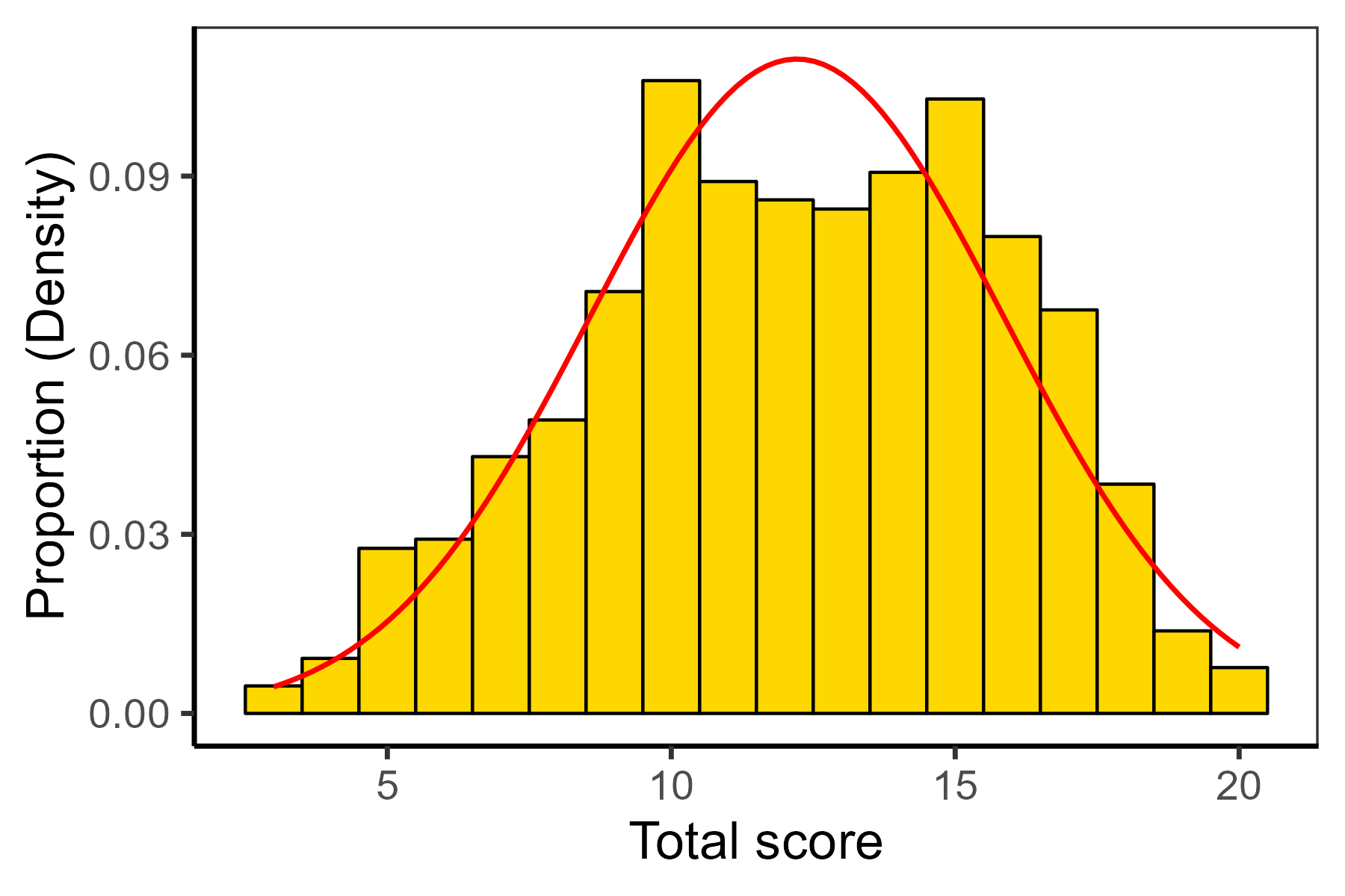
Besides the summary statistics, the histogram of the total scores might be plotted to describe their distribution (Figure 1.4, see Supplementary R code).

In R, the Z-score and T-score can be easily calculated using the scale() function. The as.vector() function is used here to convert the data frame into a vector. Besides these standardized values, the success rate can be computed as a simple function of the maximum score obtained.

(zscore <- as.vector(scale(HCI$total)))[1:7]
[1] 1.040755 1.865002 1.315504 2.139751 1.865002 2.139751 2.139751
(tscore <- 10 * zscore + 50)[1:7]
[1] 60.40755 68.65002 63.15504 71.39751 68.65002 71.39751 71.39751
(success_rate <- 100 * (HCI$total / max(HCI$total)))[1:7]
[1]  80  95  85 100  95 100 100

The first respondent in the HCI dataset scored 16 points out of 20, which corresponds to a Z-score of 1.04, i.e., approximately 1 SD above the mean. This further corresponds to the T-score of 60.41 points, and to the success rate of 80%.

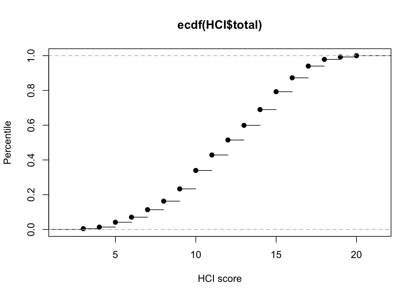
Respondent’s outcome can also be presented as a percentile enumerating the percentage of respondents who received a given score or lower. In R, the percentiles may be computed with the ecdf() function, standing for empirical cumulative distribution function. We display the function returned by the ecdf() using the plot() method (Figure 1.1). To obtain percentiles, we simply enumerate this function for values of respondents’ scores HCI$scores and multiply by 100; the original values are rounded with the round() function.

plot(ecdf(HCI$total), xlab = "HCI score", ylab = "Percentile")
Figure 1.1: Empirical cumulative distribution of HCI total scores.
ecdf(HCI$total)(HCI$total)[1:7]
[1] 0.8725038 0.9923195 0.9400922 1.0000000 0.9923195 1.0000000 1.0000000
(percentiles <- round(100 * ecdf(HCI$total)(HCI$total)))[1:7]
[1]  87  99  94 100  99 100 100

The first respondent is placed on the 87th percentile, meaning that their score is the same or higher than the scores of 87% of all respondents. Contrarily, the fourth respondent received a full score of 20 points, placing them in the 100th percentile.

1.5.3 Covariates and more complex data structures

Besides item scores coming from an instrument of interest, a number of covariates may be present in the data. Generally, any binary, ordinal, nominal, or continuous characteristics of respondents, raters, or items may be analyzed together with item responses in more complex models. These include respondent or rater age, gender, and proficiency, or the topical category of an item.

Criterion variables are covariates which are typically used for getting proofs of measurement criterion validity (Chapter 2), or item criterion validity (Chapter 5). For an educational test, a criterion variable may be the score on a different educational test, a final grade or grade-point average, or a binary variable describing current or future study success. In the case of a newly developed health-related or psychological measurement, a score from an existing, gold standard assessment may be used as a criterion variable.

Structural variables describe hierarchical structure of the data. For example, in national tests or international large scale assessments, the students are clustered within classes which are clustered within schools; these are then clustered within towns, counties, and countries. Structural variables can be included into a model to account for such a hierarchical structure, and they allow for the analysis of differences between clusters and calculations of expected values for different levels of hierarchies.

More complex data structures are possible. One complexity that may arise is from multiple time points yielding longitudinal item data. Data from a number of instruments may be available, and the relationships between them may require an additional study. Yet another complexity that may arise is in the case of adaptive testing (see Chapter 10) when items are presented in a different order to the respondents. Other more complex data structures can be considered as well.

Covariates in R. To explore relationships between binary item scores and a categorical criterion variable, a contingency table summarizing correct and incorrect responses may be displayed with respect to a discrete criterion variable. For example, in the HCI dataset, the counts of correct and incorrect answers may be computed based upon a variable major, describing whether or not the student plans to major in science. This can be done by again using the table() function and the criterion variable as the second variable in the function argument. In the output, rows represent the first variable, i.e., responses to item 1, while the columns describe the second variable, i.e., whether a student plans to major in science.

table(HCI$"Item 1", HCI$major)
   
      0   1
  0  97  99
  1 168 287

There were 99 students who are planning to major in science but who did not answer the first item correctly, while there were 287 students who plan to major and answered correctly.

The proportions of correct answers by major may again be displayed using the proportions() or prop.table() functions. The argument margin specifies whether the proportions are calculated by rows (margin = 1) or by columns (margin = 2).

proportions(table(HCI$"Item 1", HCI$major), margin = 2)
   
            0         1
  0 0.3660377 0.2564767
  1 0.6339623 0.7435233

Respondents who were planning to major in science had a slightly higher ratio of correct answers (0.74) in item 1 than respondents not planning to major in science (0.63).

To explore item response patterns in nominal items with respect to their group, one may again use the table() function and the grouping variable as the second additional argument, and, proportions may be displayed with the proportions() or prop.table() functions. Alternatively, summary statistics can also be displayed by group using the by() function and corresponding FUN argument.

table(HCItest$gender, HCItest$"Item 1")
   
      A   B   C   D
  0  16  34  65 290
  1  11  25  45 165
proportions(table(HCItest$gender, HCItest$"Item 1"), margin = 1)
   
             A          B          C          D
  0 0.03950617 0.08395062 0.16049383 0.71604938
  1 0.04471545 0.10162602 0.18292683 0.67073171
by(HCI$"Item 1", HCI$gender, FUN = summary)
HCI$gender: 0
   Min. 1st Qu.  Median    Mean 3rd Qu.    Max. 
  0.000   0.000   1.000   0.716   1.000   1.000 
------------------------------------------------------------ 
HCI$gender: 1
   Min. 1st Qu.  Median    Mean 3rd Qu.    Max. 
 0.0000  0.0000  1.0000  0.6707  1.0000  1.0000 

In the HCItest dataset, we see that male respondents (gender = 0) chose slightly more often the correct option D in item 1 while females (gender = 1) chose slightly more often all the other options in this item. This corresponds to the scored binary HCI dataset, where the male respondents had a slightly higher ratio of correct answers (a higher mean item score) in item 1 than females.

1.6 Modeling measurement data

In the sections above, we discussed how different measurement data types can be explored with descriptive statistics. In this section, we will discuss the modeling approach, in which the observed value is assumed to be a random realization of a random variable with some underlying distribution. This modeling approach is a very important step which will allow us to make statistical inferences. This approach will also give us the possibility to simulate measurement data and learn more about the properties of different modeling methods. Besides modeling the measurement data, theoretical distributions may be used to enumerate our prior beliefs about the data or about the model parameters, and such beliefs can be further used in Bayesian modeling to calculate the posterior distributions which account for the observed data.

The normal distribution is the most common distribution. It became better known with the work of Gauss; thus it is also called the Gaussian distribution. We use the notation \(X \sim \mathcal{N}(\mu, \sigma^2)\) to say we assume that the random variable \(X\) has a normal distribution with a mean of \(\mu\) and a variance of \(\sigma^2\), defined by formulae in Appendix C.

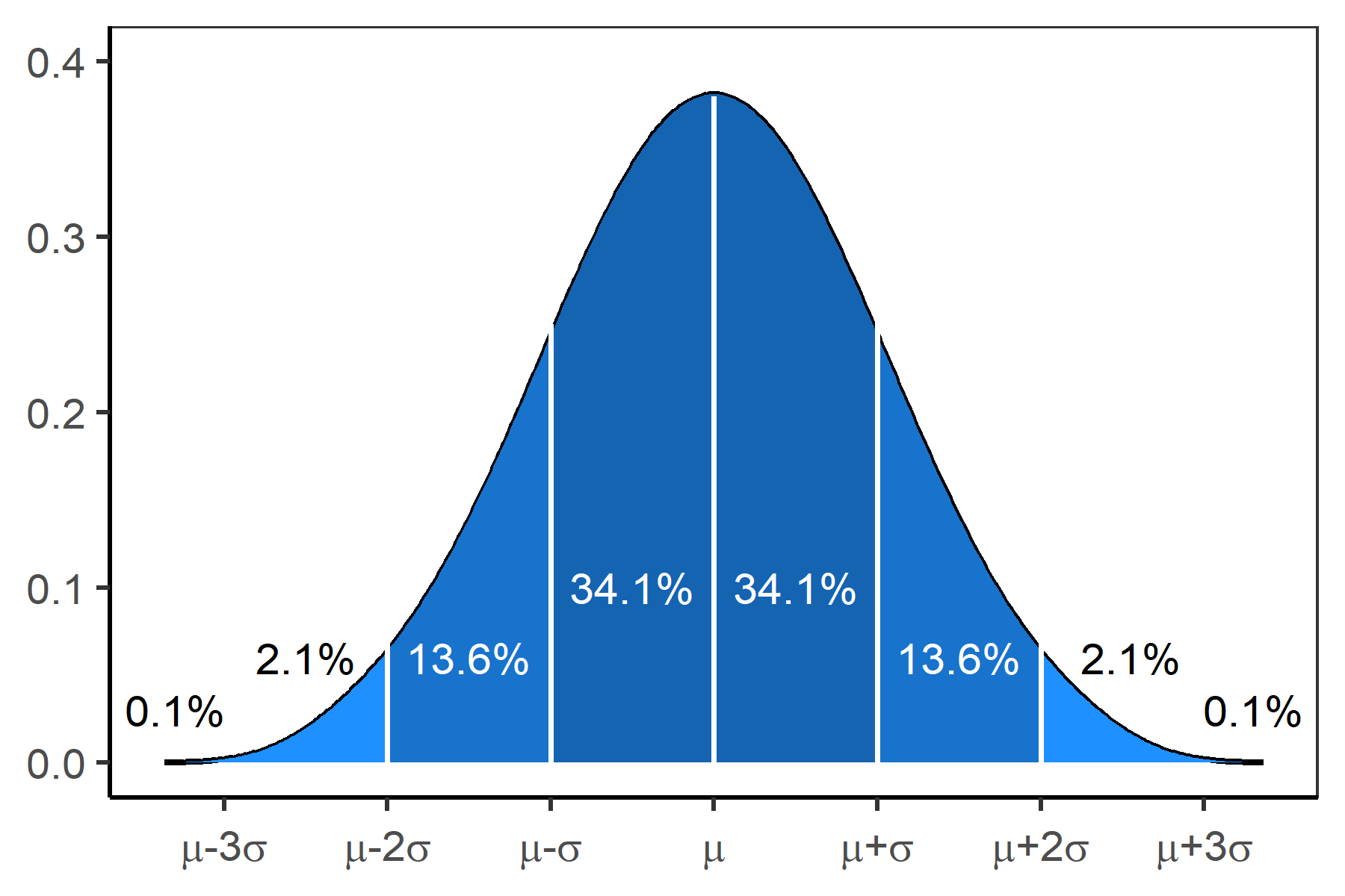
An important property of normal distribution is the so-called 68–95–99.7 rule. It states that for normally distributed random variables with a population mean \(\mu\) and standard deviation \(\sigma\), approximately 68%, 95% and 99.7%, respectively, of all values always lie 1, 2, and 3 standard deviations from the mean (Figure 1.2).

Figure 1.2: The 68–95–99.7 rule for the normal distribution.

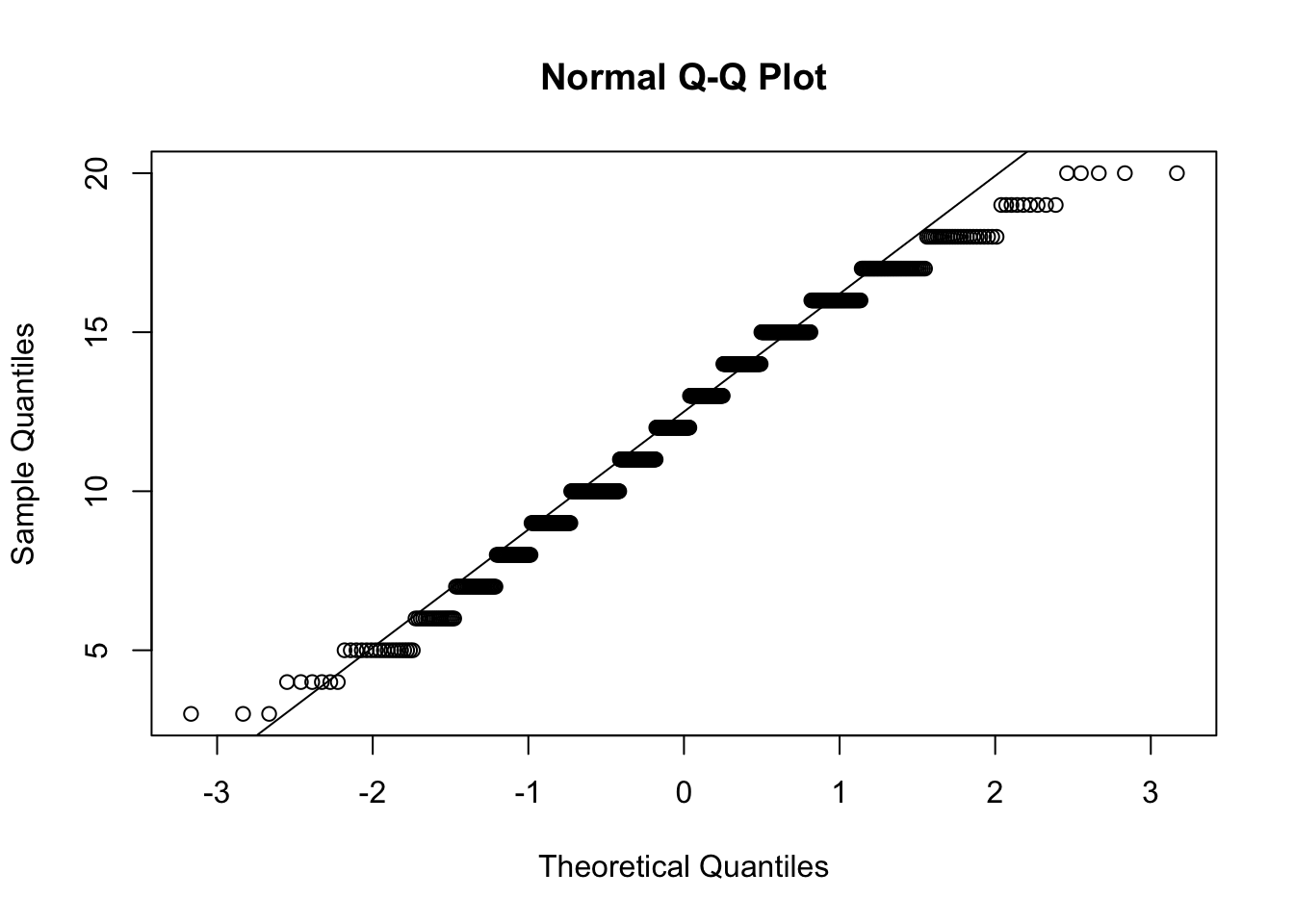
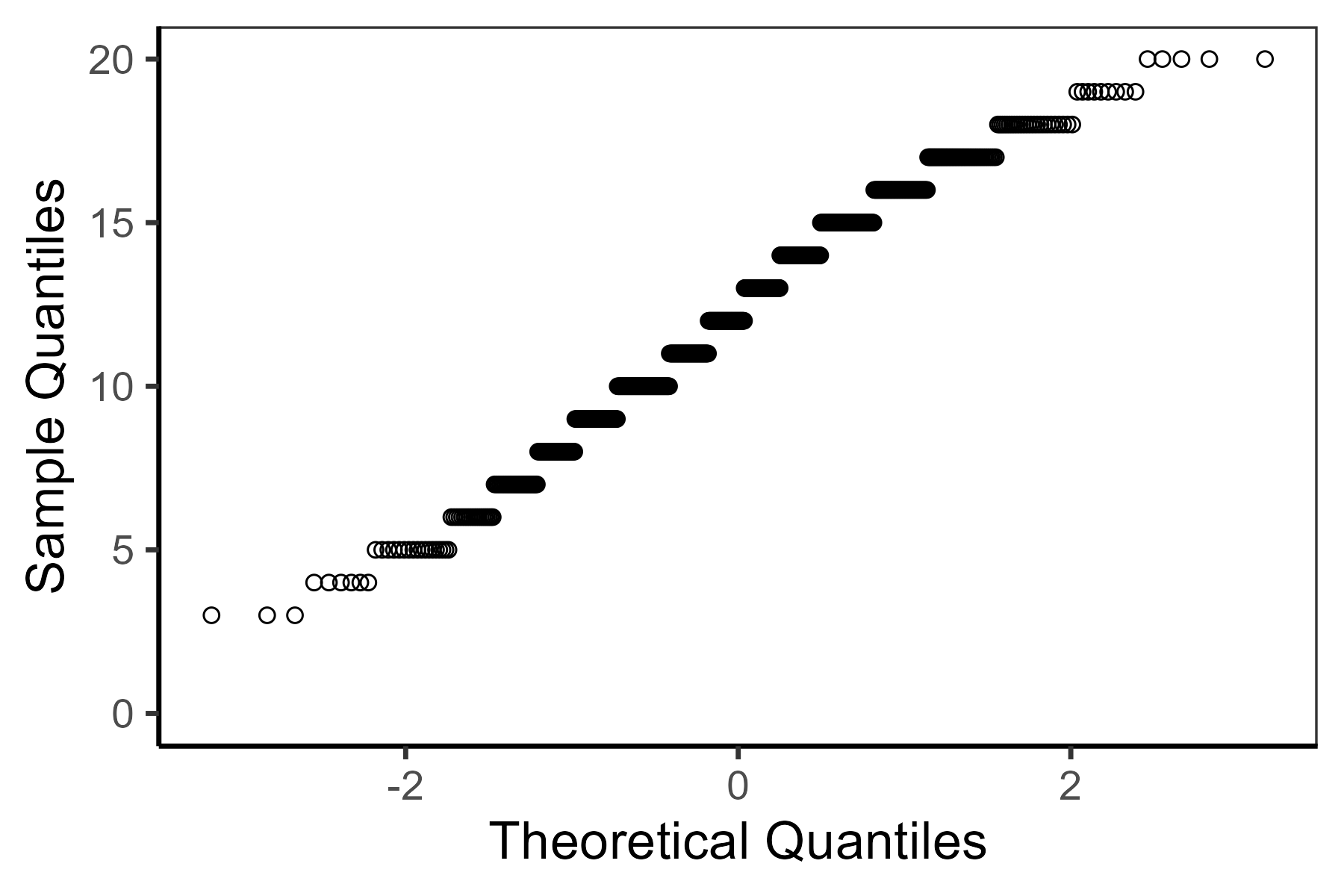
The assumption of normal distribution is a very common one. A number of methods and models that we present in this book assume that the variables are normally distributed. To what extent this assumption is plausible can be visually checked when plotting the histogram, or when formally using statistical tests of normality. One possibility is to accompany a histogram with a hypothetical normal distribution with the mean and standard deviation estimated from the data. Another option is to check the alignment to a linear line in the QQ plot depicting the sample quantiles against the theoretical quantiles of the theoretical (normal) distribution.

There are several other distributions which we will be using throughout the book; see Appendix C for more details.

Normal distribution in R. The 68–95–99.7 rule (Figure 1.2) can be checked using the qnorm() function, which provides quantiles for the normal distribution. For example, assuming that the variable of interest has a standard normal distribution, 95% of its values fall between the 2.5th and 97.5th quantile:

qnorm(0.975)
[1] 1.959964
qnorm(0.025)
[1] -1.959964

In other words, 95% of the values fall within the interval of (−1.96, 1.96) which is roughly 2 standard deviations from the mean. This property is very important for enumerating the 95% confidence intervals of parameter estimates, and we will be using this property throughout the book.

To illustrate checking for normality of the real data, we use scores from the HCI dataset and the ggplot2 package with its ggplot() and geom_histogram() functions to plot the histogram. We use the stat_function() to add the fitted normal density function into the plot (see Supplementary R code). We also use the base qqnorm() and qqline() functions to plot the QQ plot and the respective linear line.

qqnorm(HCI$total)
qqline(HCI$total)
Figure 1.3: QQ plot of HCI total scores.
(a) Histogram with fitted normal distribution density function
(b) QQ plot
Figure 1.4: Normality assumption visual check for the HCI total scores.

The plots in Figure 1.4 confirm approximately normal distribution, with a slightly negative skew and with a slightly lower kurtosis. Multiple peaks may signalize that the data is a mixture of different subgroups (also see Section A.5).

1.7 ShinyItemAnalysis interactive application

Throughout the book we employ an interactive application which is part of the ShinyItemAnalysis package. It was created with the intent to support the teaching of psychometric concepts and to help enforce complex psychometric analysis in the validation process. The interactive ShinyItemAnalysis application is available online at:

https://shiny.cs.cas.cz/ShinyItemAnalysis

and also at some mirror pages.

It is also possible to run the application locally in R using the run_app() function of the ShinyItemAnalysis package.

ShinyItemAnalysis::run_app()

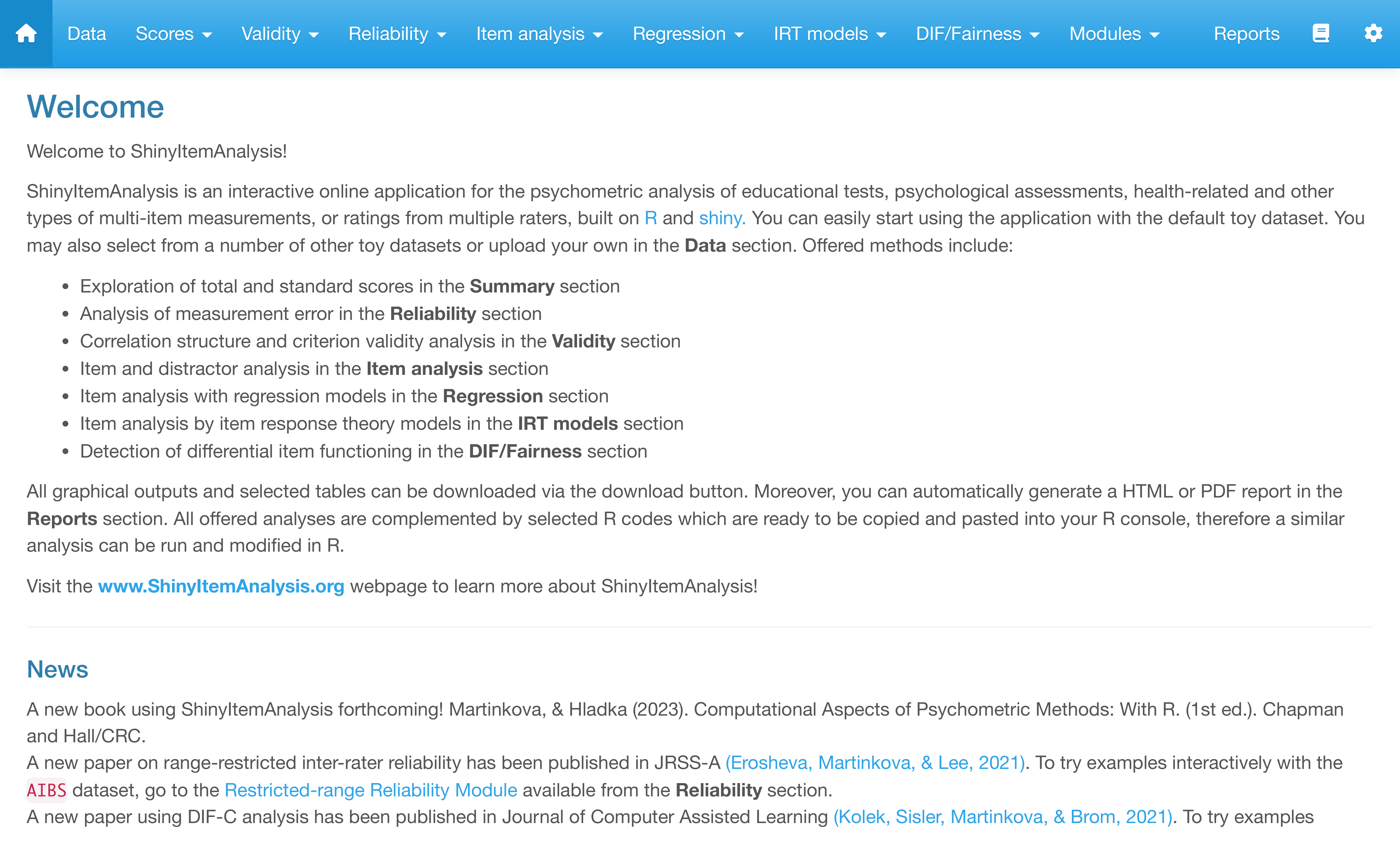
The interactive, user-friendly environment offers a number of toy datasets, as well as the possibility to upload the user’s own data. Various tools are included in separate tabs with logical ordering into separate sections, which we will discuss separately in the following chapters: Validity (Chapter 2 and Chapter 3), reliability (Chapter 4), traditional item analysis (Chapter 5), regression models for item description (Section 9.4), IRT models (Chapter 7 and Chapter 8), and differential item functioning analysis (Chapter 9). It is also possible to add new ShinyItemAnalysis modules to cover a specific topic in detail (Chapter 10). Finally, the last tab allows for the automatic generation of HTML and PDF reports. Each of the tabs includes a sample R code, which can be directly copied and pasted in the R console, and further adapted to explore the methods on different datasets or with different settings.

Figure 1.5: Intro page of the ShinyItemAnalysis interactive application.

1.8 Summary

In this chapter, we have presented a brief history of psychometrics, as well as an overview of the measurement process in different areas of social sciences with focus on education, psychology, and health. We have then presented measurement data used in this book and provided an introduction to psychometrics with R. We have further focused on exploration of measurement data with descriptive statistics, and on modeling measurement data with probabilistic models, while details on these introductory topics were left for Appendices. The final section introduced the interactive application of the ShinyItemAnalysis package.


  1. https://www.ets.org/toefl/↩︎

  2. https://englishtest.duolingo.com/↩︎

  3. https://collegeboard.org/sat/↩︎

  4. https://www.aamc.org/mcat/↩︎

  5. https://gamsat.acer.org/↩︎

  6. https://www.mba.com/exams/gmat/↩︎

  7. https://ilsa-gateway.org/↩︎

  8. https://www.who.int/standards/classifications/↩︎

  9. https://www.healthmeasures.net/↩︎