8 More on IRT
8.1 Introduction
The IRT models introduced in Chapter 7 assumed binary items and a single underlying latent trait. However, many measurement instruments involve categorical items with a higher number of categories, rating scales implementing Likert-scale questions, partial-credit items, or multiple-choice questions. Some instruments measure multiple traits or more complex structures: For example, the BFI is designed to assess five general personality traits, which are further described by more detailed latent trait facets. In this case, simultaneous estimation of these latent traits may be of interest.
In this chapter, we relax some of the earlier assumptions of the IRT models. We first present generalizations for polytomous items, both ordinal and nominal. We then focus on IRT models for multiple latent traits, and we describe multidimensional IRT models extending the models for binary and polytomous items. Both the exploratory and the confirmatory models are presented. Finally, we present estimation methods for the more complex models and algorithms which may speed up the computations.
8.2 IRT models for polytomous items
We will first present generalizations of the binary IRT models for ordinal and nominal items. The models considered in this section are latent variable counterparts of generalized linear models using cumulative logits, adjacent-categories logits, or baseline-category logits presented in Section 9.4. We will also discuss how additional restrictions on item parameters may be implemented. For a more intensive overview of the presented polytomous IRT models, the reader is referred to Nering & Ostini (2011) and Linden (2017).
8.2.1 Cumulative logit IRT models
Cumulative logit IRT models are appropriate for modeling ordinal items, such as items rated on a Likert scale. The cumulative response models are especially helpful for situations where one is interested in the probabilities of gaining at least a certain cut-score \(k\). These models are IRT counterparts to the cumulative logit regression model Equation 6.18.
8.2.1.1 Graded response model
The GRM (Samejima, 1969) uses the 2PL IRT model Equation 7.3 to describe cumulative probabilities. We assume \(K_i + 1\) categories \(k = 0, \dots, K_i\) for item \(i\), meaning each item may have a different number of ordered categories. The probability of gaining at least \(k\) points, given the respondent’s \(p\) latent ability level \(\theta_p\) is modeled as \[ \pi^{*}_{pik} = \Pr(Y_{pi} \geq k|\theta_p) = \frac{\exp\left(a_i(\theta_p - b_{ik})\right)}{1 + \exp\left(a_i(\theta_p - b_{ik})\right)}, \quad k = 1, \dots, K_i, \tag{8.1}\] with \(a_i\) being the item-specific slopes and \(b_{ik}\) being the category-specific difficulty parameters of item \(i\). In other words, \(b_{ik}\) are the locations of inflection points for the cumulative probability functions which are ordered by the category index \(k\), i.e., \(b_{i1} < b_{i2} < \dots < b_{iK_i}\). See Figure 8.1 (a) for a hypothetical example. For the first category \(k = 0\), the cumulative probability is \(\pi^{*}_{pi0} = 1\).
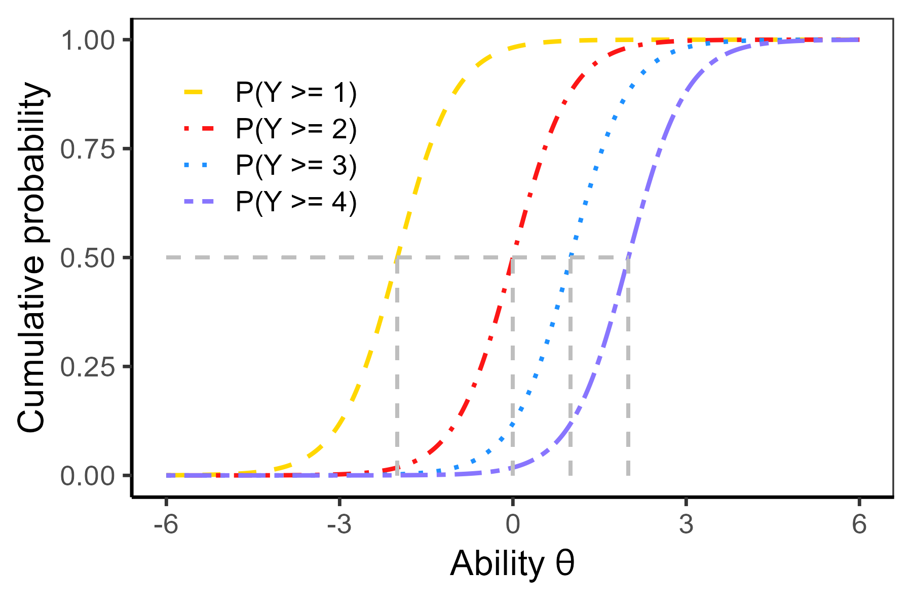
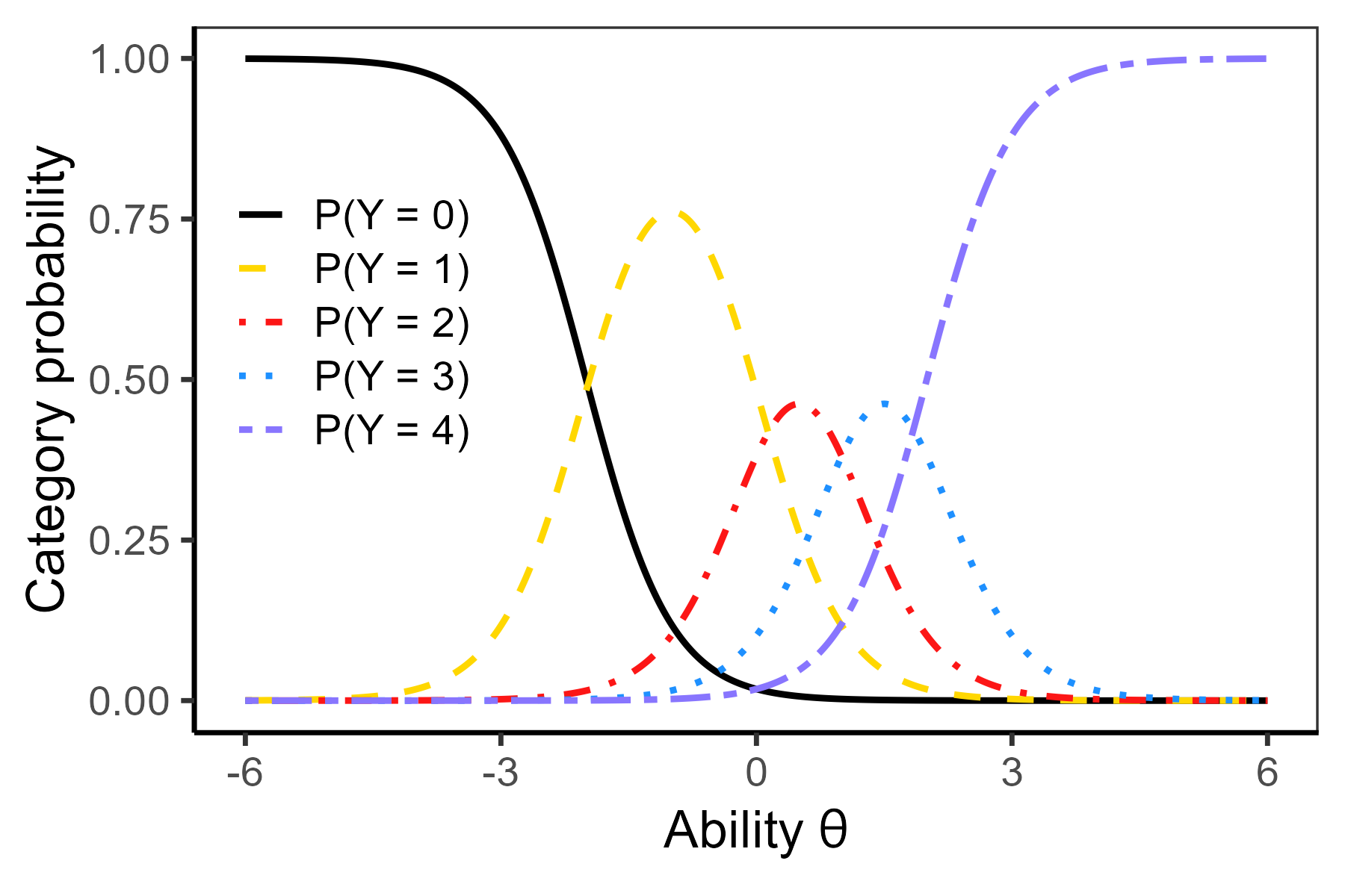
The category probability, i.e., the probability that an item response is exactly \(k\), is calculated simply as the difference between two cumulative probabilities: \[ \pi_{pik} = \Pr(Y_{pi} = k|\theta_p) = \pi^{*}_{pik} - \pi^{*}_{pi(k + 1)}, \quad k = 0, \dots, K_i - 1, \] while for the last category \(k = K_i\) of item \(i\) the category probability is equal to the cumulative probability, \(\pi_{piK_i} = \pi^{*}_{piK_i}\), since there is no higher category. Item response category probabilities may be plotted as category probability curves; the software sometimes uses the term IRC. Note that the category difficulty parameters \(b_{ik}\) are not necessarily the locations of the category intersections (Figure 8.1 (b)).
From Equation 8.1 it follows that the GRM assumes a linear form of cumulative logits: \[ \text{logit}(\pi^{*}_{pik}) = \log\left(\frac{\pi^{*}_{pik}}{1 - \pi^{*}_{pik}}\right) = a_i(\theta_p - b_{ik}), \quad k = 1, \dots, K_i; \] therefore, it is a GLMM with a cumulative logit link function. Note that when there are only two response categories 0 and 1, the model reduces to the 2PL IRT model Equation 7.3.
The model is typically fitted in the intercept-slope parametrization \[ \text{logit}(\pi^{*}_{pik}) = \beta_{0ik} + \theta_p\beta_{1i}. \] Parameters in the IRT parametrization Equation 8.1 are calculated using Equation 6.19 as \(a_{i} = \beta_{1i},\) and \(b_{ik} = -\beta_{0ik}/\beta_{1i}\). Corresponding standard errors are computed using the delta method Equation 6.10.
Assuming that the variance of the latent variable \(\theta\) is fixed (it is typical to assume that \(\theta \sim \mathcal{N}(0, 1)\), thus the variance being fixed at 1), the GRM will estimate \(m\) slope parameters and \(\sum_{i = 1}^m K_i\) location parameters, that is \(\sum_{i = 1}^m (K_i + 1)\) parameters in total. This makes \(m (K + 1)\) in the case of an equal number of \(K_i + 1 = K + 1\) categories for all items. If the latent ability variance is freely estimated, one of the item location parameters is typically fixed, or the sum of the locations might be set to 0.
GRM in the mirt package. To demonstrate how ordinal IRT models can be fitted in R, we use the Anxiety dataset. We work only with the first 29 columns describing item responses.
data("Anxiety", package = "ShinyItemAnalysis")
head(Anxiety_items <- Anxiety[, paste0("R", 1:29)], n = 2)
##   R1 R2 R3 R4 R5 R6 R7 R8 R9 R10 R11 R12 R13 R14 R15 R16 R17
## 1  1  1  1  1  1  1  1  2  2   1   2   2   1   1   1   1   1
## 2  1  1  1  1  1  1  1  1  1   1   1   1   1   1   1   1   1
##   R18 R19 R20 R21 R22 R23 R24 R25 R26 R27 R28 R29
## 1   2   1   2   2   1   1   2   3   2   1   1   2
## 2   1   1   1   1   1   1   1   2   1   1   1   1
In the mirt package, the main function mirt() may be used to fit GRM using the argument itemtype = "graded". Other options and arguments are the same as when using the mirt() function for fitting dichotomous items, see Section 7.4.1. The unidimensional model is specified with the argument model = 1. As in the case of binary items, the argument SE = TRUE is needed to enforce calculation of a variance/covariance matrix for later calculations of standard errors or confidence intervals of parameter estimates.
library(mirt)
fit_GRM_mirt <- mirt(Anxiety_items, model = 1, itemtype = "graded", SE = TRUE)
Estimated model parameters can be extracted using the coef() method. Intercept-slope parametrization is used as a default option. The IRT parametrization as specified in Equation 8.1 may be obtained with the argument IRTpars = TRUE. As a default, the confidence intervals of the parameters are provided. Argument printSE = TRUE needs to be used to print the standard errors (see the Supplementary R code). The output may be simplified using the argument simplify = TRUE.
coef(fit_GRM_mirt, IRTpars = TRUE, simplify = TRUE)
## $items
##         a     b1    b2    b3    b4
## R1  3.449  0.494 1.251 2.031 2.814
## R2  3.168  0.568 1.426 2.253 3.253
## ...
## R25 1.372 -0.762 0.154 1.377 2.592
## ...
Item 1 “I felt fearful” has a higher value of estimated discrimination and higher difficulties than item 25 “I had difficulty sleeping”. For example, as can be read from the b2 estimates, an anxiety level of 1.25 is needed to feel fearful at least “Sometimes” with a probability of 0.5, while a much lower anxiety level of only 0.15 is needed to have difficulty sleeping at least “Sometimes” with the same probability.
The TIC and TSC, as well as the IRC, the ICC, and the IIC for each item may be plotted using the plot() method or the itemplot() function applied to the resulting model. We display here the IRCs with the plot() method for items 1 and 25 by specifying the argument type = "trace" and argument which.items. See the Supplementary R code for generating the other plots.
plot(fit_GRM_mirt, which.items = c(1, 25), type = "trace")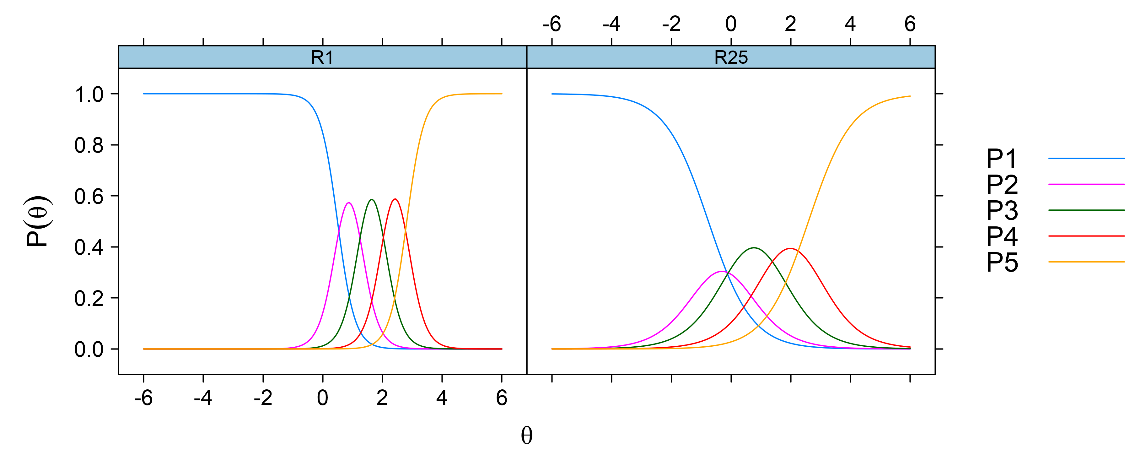
Anxiety dataset in the mirt package. Left: Item R1 “I felt fearful”. Right: Item R25 “I had difficulty sleeping”.
There are apparent differences in the slopes of the two items, as well as in the predicted probabilities of the different response options. Based upon the data, the model predicts some sleeping difficulties will be reported even by the respondents with an average level of anxiety (right part of Figure 8.2). Feeling fearful sometimes or even more often is expected to be reported by only those respondents with higher levels of anxiety (left part of Figure 8.2).
Latent ability estimates can be computed using the methods presented in Section 7.3.4.1 with the fscores() function. The argument full.scores.SE = TRUE needs to be added to print the standard errors.
fsSE <- fscores(fit_GRM_mirt, full.scores.SE = TRUE)
head(fsSE, n = 2)
##           F1  SE_F1
## [1,] -0.1426 0.1618
## [2,] -1.4172 0.4356
The first respondent’s level of anxiety is estimated to \(0.14\) (SE = 0.16), meaning their level of anxiety is 0.14 standard deviations below average. The second respondent’s anxiety is even lower, about \(1.42\) (SE = 0.44) standard deviations below average.
GRM in the ltm package. In the ltm package, the GRM may be fitted using the grm() function. Available function options, printing coefficients with the coef() method, and plotting are analogous to those using other IRT models within this library, see Section 7.4.2.
library(ltm)
fit_GRM_ltm <- grm(Anxiety_items)
coef(fit_GRM_ltm)
##     Extrmt1 Extrmt2 Extrmt3 Extrmt4 Dscrmn
## R1    0.560   1.461   2.366   3.325  2.773
## R2    0.657   1.667   2.604   3.741  2.605
## ...
## R25  -0.918   0.150   1.612   3.056  1.153
## ...
Item parameters differ only slightly from those obtained when using the mirt package.
For each item, the cumulative response curve, the IRC, and the IIC can be plotted using the plot() method, by specifying the argument type as either "OCCu" (software uses the term “operation characteristic curve” instead of “cumulative response curve”), "ICC", or "IIC". We display here the cumulative response curves and the IRCs for item 25 by specifying the argument items = 25.
plot(fit_GRM_ltm, type = "OCCu", items = 25)
plot(fit_GRM_ltm, type = "ICC", items = 25)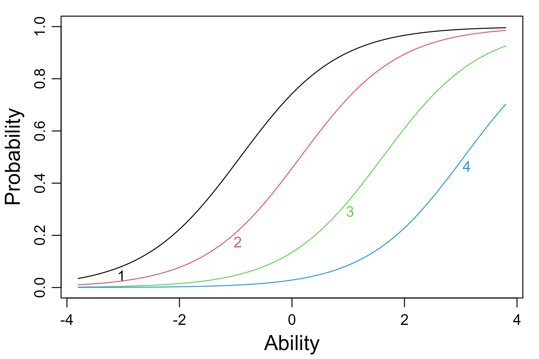
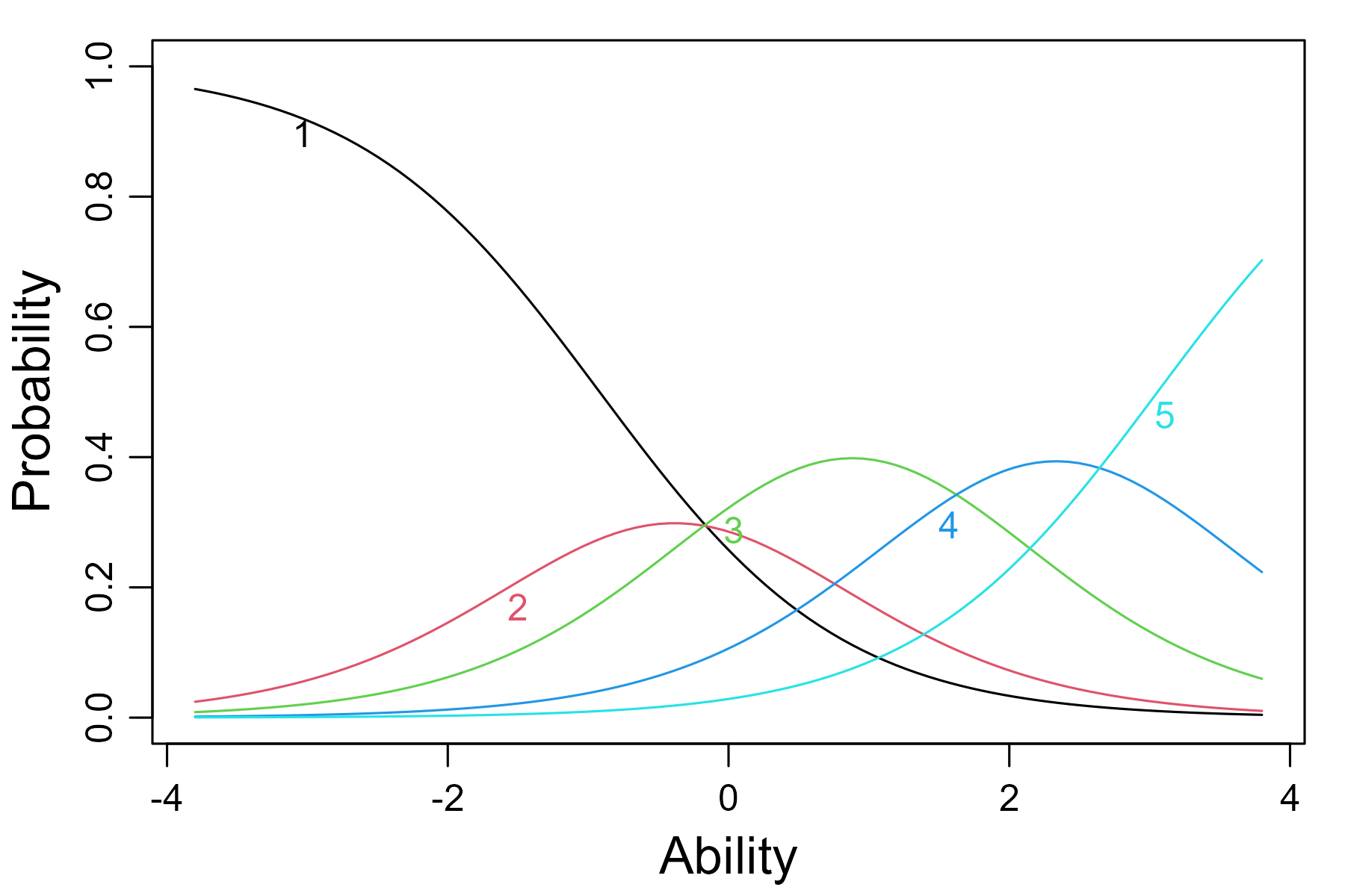
Anxiety dataset in the ltm package.
The IRCs plotted with the ltm package (Figure 8.3 (b)) are similar to those plotted with the mirt package (right part of Figure 8.2).
Latent abilities, i.e., factor scores, can be computed using the factor.scores() function. We declare the name of the package directly to prevent issues due to duplication in the function name – a function of the same name is present in the psych package. Various estimation methods (see Section 7.3.4.1) may be specified with the argument method; the default option is empirical Bayes (method = "EB"). Recall that, by default, the ltm package returns the factor scores for all uniquely observed response patterns. To calculate the factor scores for all respondents, the actual response patterns need to be specified with the argument resp.patterns.
ltm::factor.scores(fit_GRM_ltm, resp.patterns = Anxiety_items)
## Factor-Scores for specified response patterns:
## R1 R2 ... R22 R23 R24 R25 R26 R27 R28 R29 Obs   Exp     z1 se.z1
## 1   2 ...   1   2   2   1   1   2   3   2   0 0.000 -0.012 0.183
## 2   2 ...   1   1   1   1   1   1   2   1   0 0.011 -0.933 0.300
## 3   2 ...   1   1   1   1   1   1   3   2   0 0.000  0.025 0.186
## ...
The estimated abilities are similar to those obtained from the mirt() function; for example, for the first respondent, the level of anxiety is estimated at \(-0.01\) (SE = 0.18). The two sets of ability estimates plotted against each other suggest the two functions operate similarly but not identically. The correlation between the two ability estimates is \(0.97\); the differences are due mainly to the estimation techniques used (see the Supplementary R code).
Predicted level of anxiety can also be obtained from other response patterns, which are included in the resp.patterns argument in a matrix form. We calculate below the estimated anxiety level for a hypothetical respondent who answered “Sometimes” (scored as 3) to all 29 items.
ltm::factor.scores(fit_GRM_ltm,
                   resp.patterns = t(as.matrix(rep(3, 29))))
## Factor-Scores for specified response patterns:
##     R1 ... R23 R24 R25 R26 R27 R28 R29 Obs Exp    z1 se.z1
## Exp  3 ...   3   3   3   3   3   3   3   0   0 1.751 0.139
For this hypothetical respondent, the predicted level of anxiety is quite high, about 1.75 (SE = 0.14) standard deviations above average.
8.2.1.2 Graded rating scale model
The GRSM (Muraki, 1990) is a restricted version of the GRM Equation 8.1. The GRSM assumes the same rating scale for all items. For example all items are rated on a scale “Fully disagree” – “Partly disagree” – “Partly agree” – “Agree”, or all items are rated on a scale “Never” – “Sometimes” – “Always”. The model therefore assumes the same number of \(K + 1\) categories \(k = 0, \dots, K\) for all items which are used the same way, meaning the distances between the category thresholds are the same across items. Thus, the category difficulty parameters \(b_{ik}\) in Equation 8.1 can be split into item-specific locations \(b_i\) and category-specific levels \(\lambda_k\) common to all items, so that \(b_{ik} = b_i - \lambda_k\), resulting in: \[ \pi^{*}_{pik} = \Pr(Y_{pi} \geq k|\theta_p) = \frac{\exp\left(a_i(\theta_p - (b_{i} - \lambda_k))\right)}{1 + \exp\left(a_i(\theta_p - (b_{i} - \lambda_k))\right)}, \quad k = 1, \dots, K. \tag{8.2}\] For identification purposes, the location parameter \(b_1\) for the first item is set to \(0\), or alternatively, the sum of the location parameters \(\sum b_i\) is set to \(0\). In the GRSM, the total \(2m + K - 1\) item parameters are estimated (\(m\) discrimination parameters, \(m - 1\) item location parameters, and \(K\) thresholds). This is a lower number of parameters than in the GRM, where \(m(K + 1)\) parameters are estimated. This may be of help to fit the model, especially in the case of a lower number of respondents.
GRSM in the mirt package. The GRSM with the IRT parametrization as in Equation 8.2 may be fitted using the mirt() function of the mirt package with the argument itemtype = "grsmIRT".
fit_GRSMirt_mirt <- mirt(Anxiety_items, model = 1, itemtype = "grsmIRT")
coef(fit_GRSMirt_mirt, simplify = TRUE)
##  $items
##        a1     b1     b2     b3     b4      c
## R1  3.200 -0.454 -1.256 -2.214 -3.202  0.000
## R2  3.109 -0.454 -1.256 -2.214 -3.202 -0.110
## ...
## R25 1.613 -0.454 -1.256 -2.214 -3.202  1.081
## ...
Parameter a1 is an item-specific slope \(a_i\), and parameters b1–b4 correspond to category-specific levels \(\lambda_k\), which are identical for all items. Parameter c is item-specific location \(b_i\). For identification purposes, the location parameter for the first item is fixed at c = 0.
To decide whether GRM or GRSM fits better to the Anxiety data, we can use the LRT Equation 2.29 implemented in the anova() method, or the information criteria such as AIC Equation 2.30, BIC Equation 2.31, and their modifications.
 anova(fit_GRSMirt_mirt, fit_GRM_mirt)
##        AIC     AICc    SABIC       HQ      BIC    logLik
## 1 35268.78 35279.52 35358.19 35377.76 35551.89 -17573.39
## 2 35130.82 35199.11 35343.35 35389.87 35803.79 -17420.41
##        X2  df   p
## 1     NaN NaN NaN
## 2 305.959  84   0
In this case, a p-value close to zero suggests rejecting the restricted model and keeping the larger GRM (the second line of the output). This is in line with the smaller values of the AIC and its modifications, suggesting a better fit for this less restrictive model. Notice, however, that the BIC is smaller for the GRSM, suggesting its superiority when penalizing a number of estimated parameters.
8.2.2 Adjacent-categories logit IRT models
Another option to fit the ordinal item response data is the adjacent-categories logit IRT models. These models are IRT counterparts to the adjacent-categories logit regression model Equation 6.22. They are especially helpful when the focus is on estimating the level of ability needed to move from one category to the next one.
8.2.2.1 Generalized partial credit model
The GPCM (Muraki, 1992) fits ordinal items by assuming the 2PL IRT model for each pair of adjacent categories. In other words, a linear form is assumed for the adjacent-categories logits: \[ \log\left(\frac{\Pr(Y_{pi} = k|\theta_p)}{\Pr(Y_{pi} = k - 1|\theta_p)}\right) = \log\left(\frac{\pi_{pik}}{\pi_{pi(k - 1)}}\right) = a_i(\theta_p - b_{ik}), \quad k = 1, \dots, K_i, \tag{8.3}\] while all category probabilities add up to 1, i.e., \(\sum_{k = 0}^{K_i} \pi_{pik} = 1\), which defines the first category \(\pi_{pi0}\).
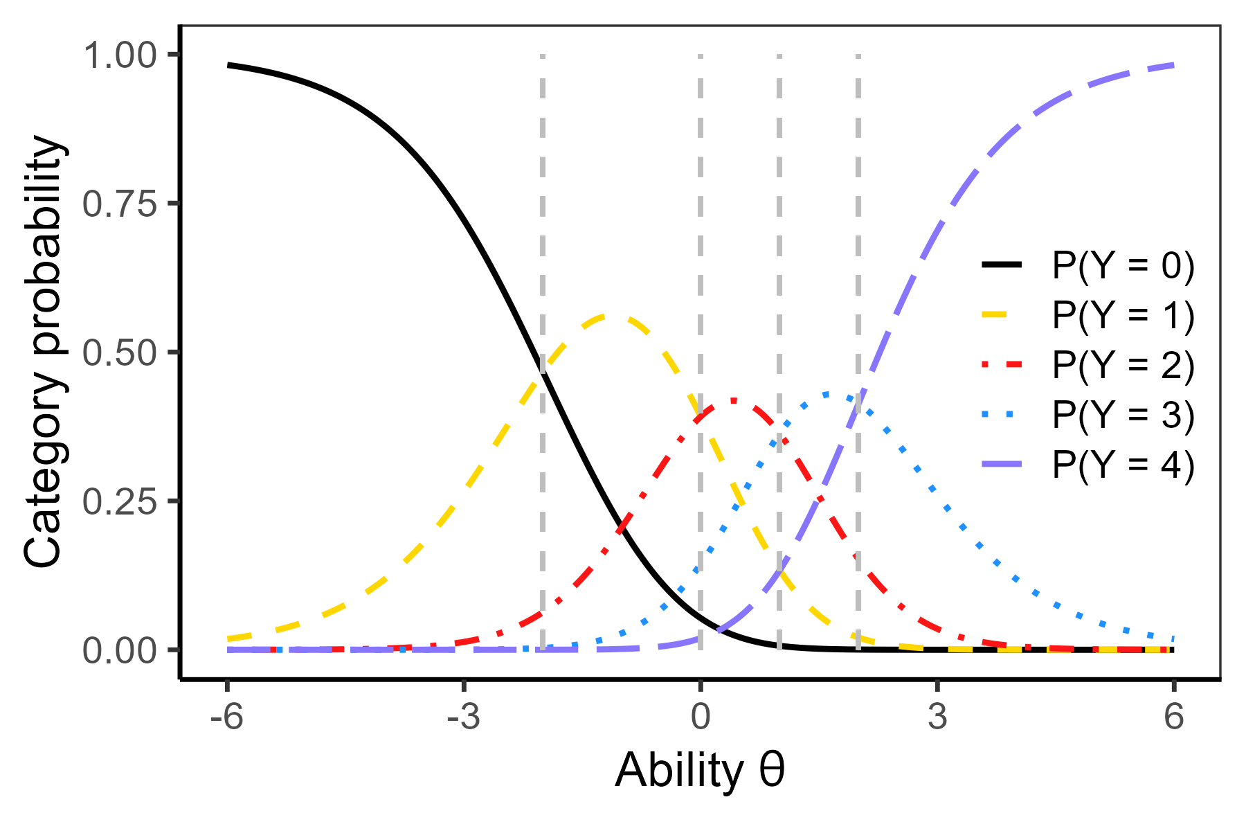
The \(b_{ik}\) are the step difficulty parameters, which represent the relative difficulty in obtaining score \(k\) over score \(k - 1.\) They can also be viewed as threshold parameters corresponding to ability levels which are needed to transition from one category into the next one. This can be seen from Equation 8.3: When \(\theta_p = b_{ik}\), the right-hand side of the equation is 0; thus \(\pi_{pik} = \pi_{pi(k-1)}\). In other words, the \(b_{ik}\) parameters describe the ability level for which the adjacent response categories intersect (Figure 8.4 (a)).
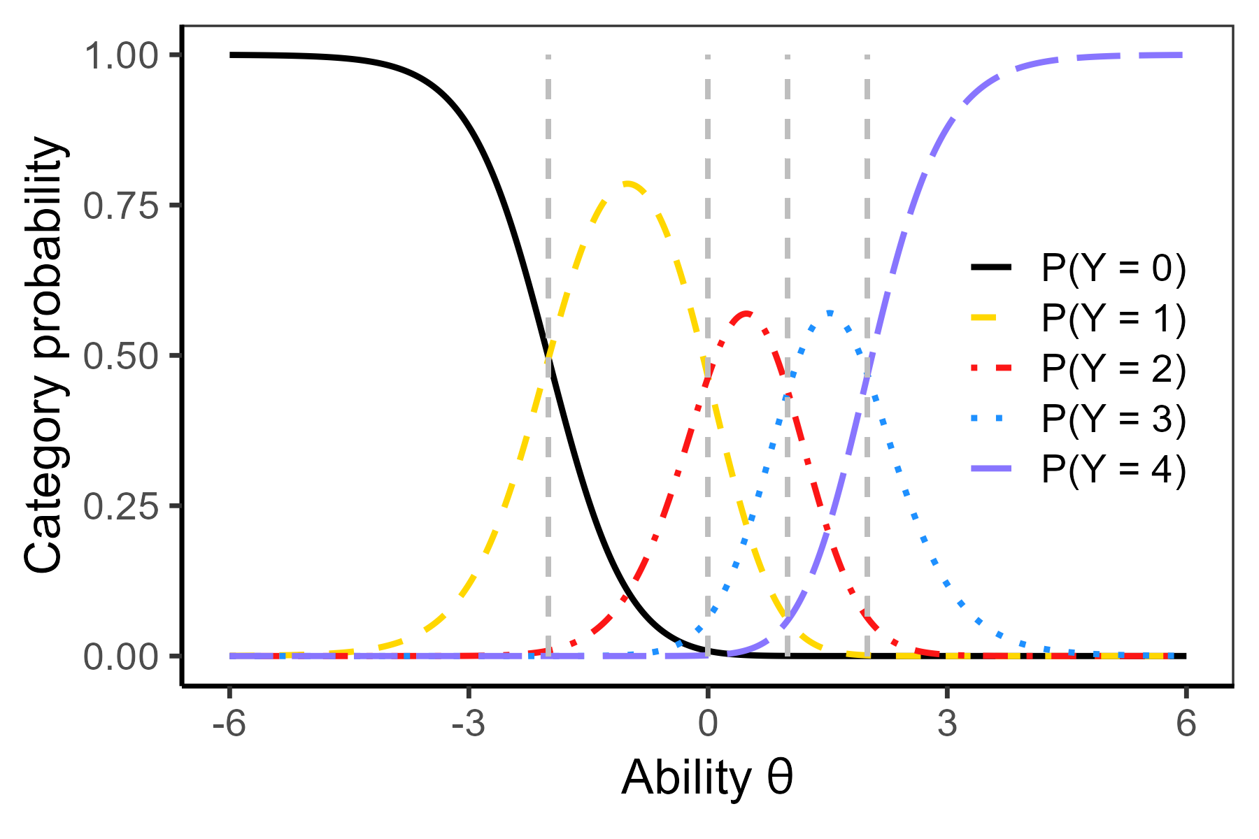
Category probabilities \(\pi_{pik}\) can be derived from Equation 8.3 (see Exercise 8.2; also see Equation 9.14 and Exercise 6.3): \[ \begin{aligned} \pi_{pik} &= \frac{\exp\left[\sum_{l = 1}^k a_i(\theta_p - b_{il})\right]}{1 + \sum_{t = 1}^{K_i}\exp\left[\sum_{l = 1}^t a_i(\theta_p - b_{il})\right]}, \quad k = 1, \dots, K_i,\\ \pi_{pi0} &= \frac{1}{1 + \sum_{t = 1}^{K_i}\exp\left[\sum_{l = 1}^t a_i(\theta_p - b_{il})\right]} = 1 - \sum_{k = 1}^{K_i} \pi_{pik}. \end{aligned} \tag{8.4}\]
Given the form of the category probabilities in Equation 8.4, the GPCM is sometimes categorized as a divide by total model. Considering the identification constraints (e.g., the variance of the abilities fixed at 1), the same number of item parameters of \(\sum_{i = 1}^{K_i}(K_i + 1)\) is being estimated as in the GRM. When there are only two response categories 0 and 1 for each item, the model reduces to the 2PL IRT model Equation 7.3 with \(2m\) item parameters.
GPCM in the mirt package. In the mirt package, the GPCM can be fitted using the mirt() function with an argument itemtype = "gpcm". We illustrate here the GPCM fitting on the Anxiety dataset.
fit_GPCM_mirt <- mirt(Anxiety_items, model = 1, itemtype = "gpcm")
coef(fit_GPCM_mirt, IRTpars = TRUE, simplify = TRUE)
## $items
##         a     b1     b2    b3    b4
## R1  2.935  0.614  1.204 1.859 2.439
## R2  2.823  0.680  1.355 2.012 2.829
## ...
## R25 0.741  0.013 -0.182 1.468 2.119
## ...
Reading from b1 estimates, in item 1 “I felt fearful”, an anxiety level of \(0.61\) was needed to move from the category “Never” to category “Rarely”, while a much lower anxiety level of \(0.01\) was needed in item 25 “I had difficulty sleeping” to prefer the category “Rarely” over “Never”. Note that in item 25, the b2 estimate was lower than b1 which may happen in adjacent-categories logit models such as GPCM.
To present further plotting functions of the mirt package, we now use the itemplot() function with an argument type = "infotrace" which provides a combined plot of IRCs and IIC.
itemplot(fit_GPCM_mirt, item = 1, type = "infotrace")
itemplot(fit_GPCM_mirt, item = 25, type = "infotrace")
The predicted category probabilities (blue lines in Figure 8.5) appear similar to those obtained from the GRM (Figure 8.2). Given the differences in the discrimination between the two items, the highest information is much larger in item 1 than in item 25 (pink lines in Figure 8.5). For item 1, the information is highest for anxiety levels close to 2, while for item 25, it is highest for those levels slightly above 0.
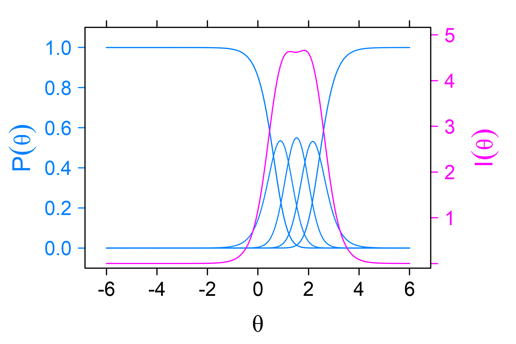
Anxiety item R1.
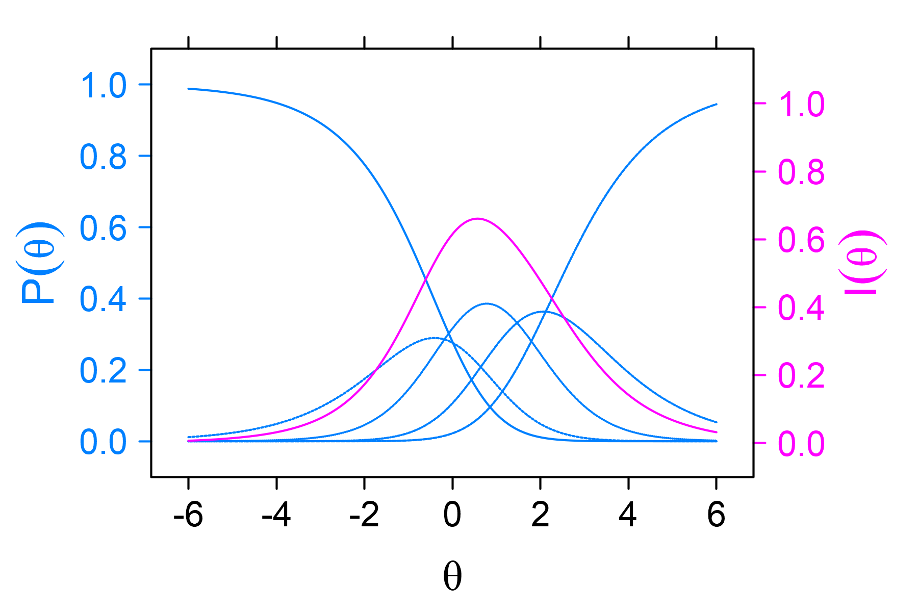
Anxiety item R25.
mirt package.
8.2.2.2 Partial credit model
The PCM (Masters, 1982) is a restricted version of the GPCM Equation 8.3. It models the log-odds of the adjacent categories \(k - 1\) and \(k\) with the 1PL model: \[ \log\left(\frac{\pi_{pik}}{\pi_{pi(k - 1)}}\right) = \theta_p - b_{ik}, \, k = 1, \dots, K_i, \] thus restricting the item slopes to \(a_i = 1\) in the GPCM Equation 8.3 and Equation 8.4. Category probabilities are then given by the equation \[ \begin{aligned} \pi_{pik} &= \frac{\exp\left[\sum_{l = 1}^k (\theta_p - b_{il})\right]}{1 + \sum_{t = 1}^{K_i}\exp\left[\sum_{l = 1}^t (\theta_p - b_{il})\right]}, \quad k = 1, \dots, K_i,\\ \pi_{pi0} &= \frac{1}{1 + \sum_{t = 1}^{K_i}\exp\left[\sum_{l = 1}^t (\theta_p - b_{il})\right]} = 1 - \sum_{k = 1}^{K_i} \pi_{pik}. \end{aligned} \tag{8.5}\] The threshold parameters \(b_{ik}\) again correspond to the intersections of the IRCs (Figure 8.4 (b)).
PCM in the mirt package. In the mirt package, the PCM model Equation 8.5 can be fitted using the mirt() function and a more general GPCM model (argument itemtype = "gpcm"), and by constraining the discrimination parameters in all of the items to a value of 1. In the following code, we demonstrate this approach on a 29-item Anxiety dataset. We specify a unidimensional model by specifying that all items load only on the single factor, F = 1-29. We declare by the FIXED argument that all slope parameters (a1) will be fixed, and we specify in the START argument the value of 1.
model_PCM <- "F = 1-29
              FIXED = (1-29, a1),
              START = (1-29, a1, 1)"
fit_PCM_mirt <- mirt(Anxiety_items, model = model_PCM, itemtype = "gpcm")
coef(fit_PCM_mirt, IRTpars = TRUE, simplify = TRUE)
## $items
##     a     b1     b2    b3    b4
## R1  1  1.305  1.948 3.184 4.106
## R2  1  1.390  2.243 3.434 4.814
## ...
## R25 1 -0.462 -0.106 1.639 2.670
## ...
The model fit of the competing models can be compared using the anova() method.
 anova(fit_PCM_mirt, fit_GPCM_mirt)
##        AIC     AICc    SABIC       HQ      BIC    logLik
## 1 36632.50 36674.32 36802.53 36839.74 37170.88 -18200.25
## 2 35326.84 35395.13 35539.37 35585.89 35999.81 -17518.42
##         X2  df   p
## 1      NaN NaN NaN
## 2 1363.662  29   0
Comparing the PCM model to a more general GPCM model, all of the information criteria as well as the LRT prefer the GPCM model, which can be read from lower criteria values in the second row and a p-value close to 0.
8.2.2.3 Rating scale model
A RSM (Andrich, 1978) further restricts the GPCM Equation 8.4 and PCM Equation 8.5. Analogously to GRSM Equation 8.2, the RSM assumes that all test items have exactly \(K + 1\) categories \(0, \dots, K\), and all items share the same rating scale structure. The threshold parameters \(b_{ik}\) are thus split into item-specific location \(b_i\) and category-specific response threshold \(\lambda_k\), i.e., \(b_{ik} = b_i - \lambda_k\).
Category probabilities Equation 8.4 are then given by \[ \begin{aligned} \pi_{pik} &= \frac{\exp\left[\sum_{l = 1}^k (\theta_p - (b_{i} - \lambda_l))\right]}{1 + \sum_{t = 1}^{K}\exp\left[\sum_{l = 1}^t (\theta_p - (b_{i} - \lambda_l))\right]} \quad k = 1, \dots, K,\\ \pi_{pi0} &= \frac{1}{1 + \sum_{t = 1}^{K}\exp\left[\sum_{l = 1}^t (\theta_p - (b_{i} - \lambda_l))\right]} = 1 - \sum_{k = 1}^{K} \pi_{pik}. \end{aligned} \] Once again, an advantage of the RSM is the lower number of parameters that are required to be estimated. With ability variance fixed to 1 and with an equal number of categories \(K_i = K\) per item, we have \(m (K + 1)\) parameters to be estimated in the GPCM, we have \(m K\) item parameters in the PCM, while we have only \(K + m - 1\) parameters in the RSM, the \(K\) threshold parameters \(\lambda_k\) and \(m\) parameters for item-specific location \(b_i\), one of which is being fixed to 0.
RSM in the mirt package. RSM can be fitted in the mirt package using the main function mirt() with the argument itemtype = "rsm":
fit_RSM_mirt <- mirt(Anxiety_items, model = 1, itemtype = "rsm")
coef(fit_RSM_mirt, IRTpars = TRUE, simplify = TRUE)
## $items
##     a1    b1   b2    b3    b4      c
## R1   1 1.347 2.09 3.797 5.101  0.000
## R2   1 1.347 2.09 3.797 5.101 -0.205
## ...
## R25  1 1.347 2.09 3.797 5.101  2.030
## ...
All items share the same slope a1 = 1 and share the same threshold parameters \(\lambda_{k}\), denoted here as b1–b4, while differing only in the item-specific location, denoted here as c, the first of which is being fixed to 0. Not surprisingly, the shapes of the IRCs and IICs for items 1 and 25 now look much more similar to each other, differing only in their horizontal location (Figure 8.6).
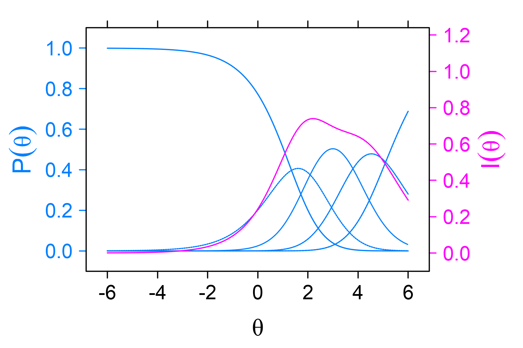
Anxiety item R1.
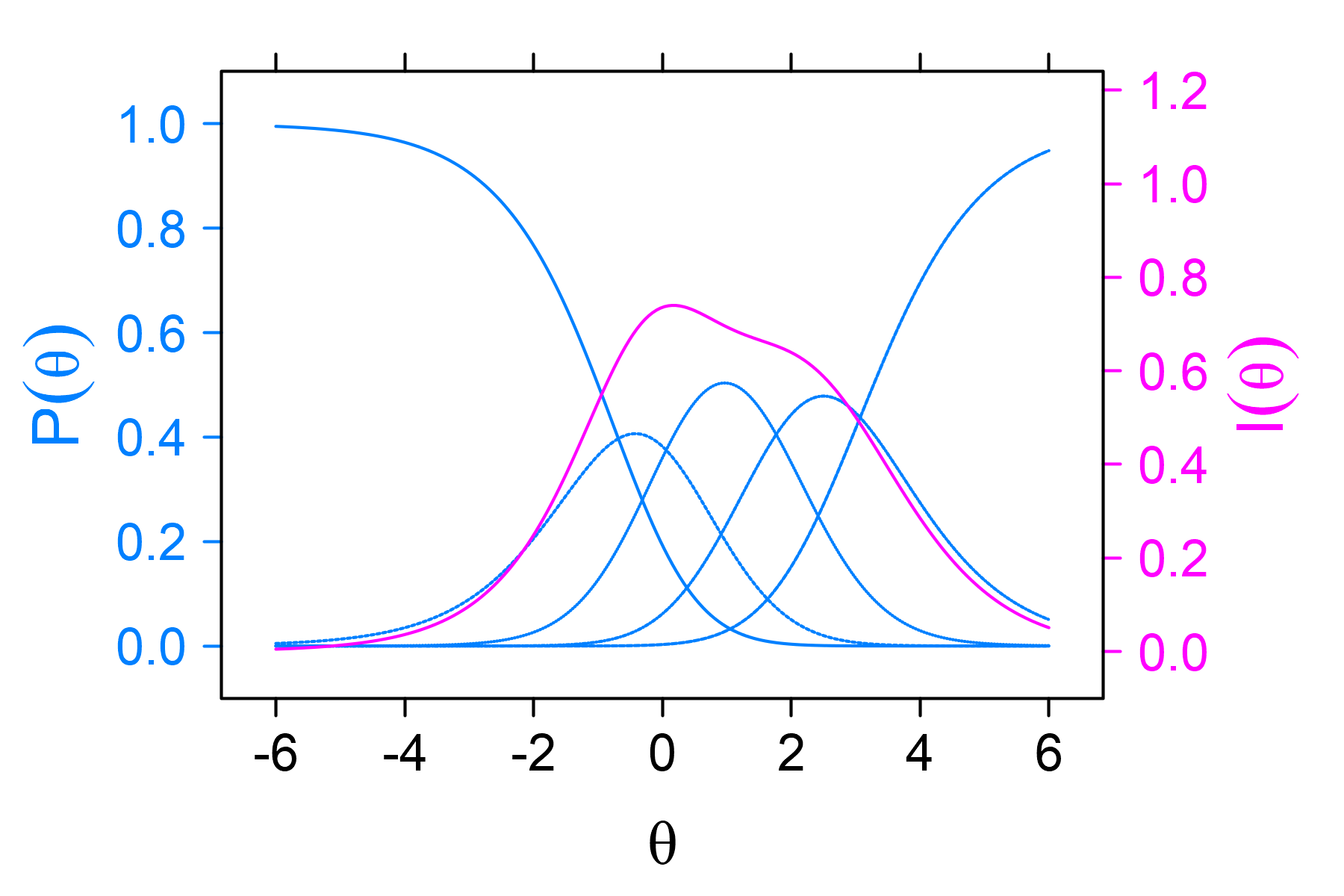
Anxiety item R25.
mirt package.
Model comparison using the anova() method suggests superiority of the richer model GPCM over the even more restrictive RSM (see the Supplementary R code).
GPCM/PCM/RSM in the ltm and eRm package.
The adjacent-categories logit IRT models may also be fitted in other packages. The gpcm() function may be used to fit the GPCM with the ltm package. An additional argument restriction = "Rasch" can be used to fit the PCM. The eRm package offers extended Rasch models, such as the PCM with the PCM() function or the RSM with the RSM() function (see the Supplementary R code for examples).
8.2.3 Baseline-category logit IRT models
We have focused so far on ordinal responses. Both the cumulative logit models (GRM, GRSM) and the adjacent-categories logit models (GPCM, PCM, RSM) provided expected ordering of the categories. In this section, we will present a model for unordered categories, the nominal responses, such as those which are present in multiple-choice items. The model is a latent variable counterpart to the multinomial regression model Equation 6.25 discussed in Section 9.4. This baseline-category logits model pairs each category with a baseline category; thus no ordering of categories is required.
8.2.3.1 Nominal response model
The NRM assumes that the baseline-category logits are following a 2PL IRT model. Using the intercept-slope parametrization we get: \[ \log\left(\frac{\pi_{pik}}{\pi_{pi0}}\right) = \beta_{0ik} + \beta_{1ik}\theta_p, \quad k = 1, \dots, K_i, \tag{8.6}\]
with \(\beta_{0ik}\) category-specific intercepts and \(\beta_{1ik}\) category-specific slopes. For identifiability reasons, a constraint needs to be added; e.g., parameters of the baseline category \(k = 0\) are fixed to zero, i.e., \(\beta_{0i0} = 0\), \(\beta_{1i0} = 0\).
Category probabilities \(\pi_{pik} = \Pr(Y_{pi} = k|\theta_p)\) are then given by: \[ \begin{aligned} \pi_{pik} &= \frac{\exp(\beta_{0ik} + \beta_{1ik}\theta_p)}{1 + \sum_{l = 1}^{K_i}\exp(\beta_{0il} + \beta_{1il}\theta_p)}, \ k = 1, \dots, K_i,\\ \pi_{pi0} &= \frac{1}{1 + \sum_{l = 1}^{K_i}\exp(\beta_{0il} + \beta_{1il}\theta_p)} = 1 - \sum_{k = 1}^{K_i} \pi_{pik}, \end{aligned} \tag{8.7}\] which follows from Equation 8.6 and from the fact that the response probabilities add up to 1, \(\sum_{k = 0}^{K_i} \pi_{pik} = 1\).
Bock’s nominal response model. Different parametrizations and identification constraints of the model may be applied. Bock’s original parametrization (Bock, 1972) was an intercept-slope parametrization Equation 8.6, which avoided selecting the baseline category. It instead assumed zero sums of the parameters: \[ \sum_{k = 0}^{K_i} \beta_{0ik} = 0, \quad \quad \textrm{and} \quad \quad \sum_{k = 0}^{K_i} \beta_{1ik} = 0. \tag{8.8}\]
Thissen’s et al. parametrization of nominal response model. Thissen et al. (2011) used intercept-slope parametrization Equation 8.6 with the parameters of the first category set to zero: \(\beta_{0i0}^{*} = 0\) and \(\beta_{1i0}^{*} = 0.\) Moreover, to allow for generalizations of multidimensional models, the authors proposed a parametrization separating an overall slope parameter \(\beta^{*}_{1i}\) while fixing the last category slope to \(\beta^{*}_{1iK_i} = K_i\). The resulting category probabilities then are as follows: \[ \begin{aligned} \pi_{pik} &= \frac{\exp(\beta_{0ik} + \beta_{1i}^{*}\beta_{1ik}^{*} \theta_p)}{1 + \sum_{l = 1}^{K_i}\exp(\beta_{0il} + \beta_{1i}^{*}\beta_{1il}^{*}\theta_p)}, \ k = 1, \dots, K_i,\\ \pi_{pi0} &= \frac{1}{1 + \sum_{l = 1}^{K_i}\exp(\beta_{0il} + \beta_{1i}^{*}\beta_{1il}^{*}\theta_p)} = 1 - \sum_{k = 1}^{K_i} \pi_{pik}. \end{aligned} \tag{8.9}\]
BL-IS and BL-IRT parametrization of nominal response model. In multiple-choice items, when information on the correct answer (key) is available, we suggest setting the correct option \(k_C\) as the baseline category, thus setting the parameters for this category to zero. With this constraint and when applying the intercept-slope parametrization, i.e., \(\beta_{0ik_C} = \beta_{1ik_C} = 0\), the NRM has the following form: \[ \log\left(\frac{\pi_{pik}}{\pi_{pik_C}}\right) = \beta_{0ik} + \beta_{1ik}\theta_p, \quad k = 0, \ \dots, K_i, \ k \neq k_C, \tag{8.10}\] which we call the BL-IS (baseline-category logit intercept-slope) parametrization.
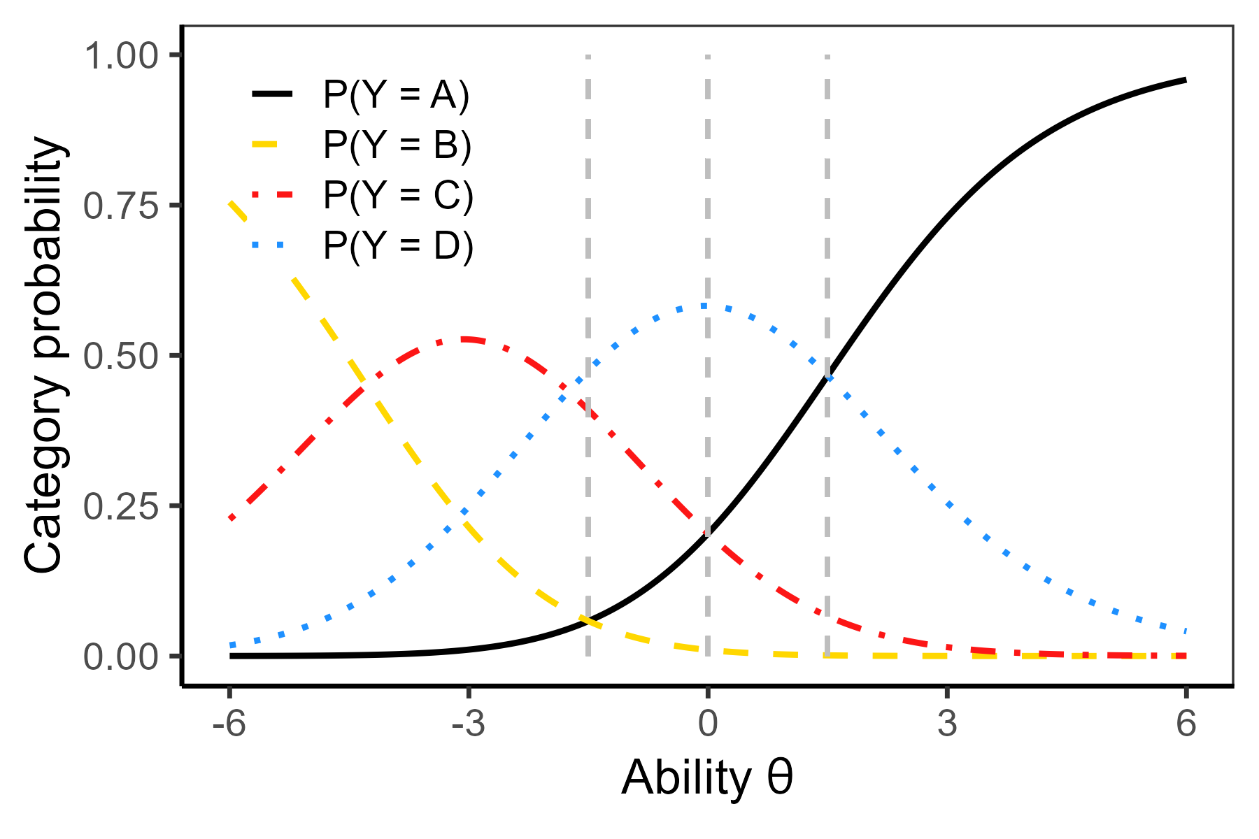
With this constraint applied together with the IRT parametrization, i.e., \(a_{ik_C} = b_{ik_C} = 0\), the NRM is given by \[ \log\left(\frac{\pi_{pik}}{\pi_{pik_C}}\right) = a_{ik}(\theta_p - b_{ik}) , \quad k = 0, \ \dots, K_i, \ k \neq k_C, \tag{8.11}\] which we call the BL-IRT parametrization. The BL-IRT parametrization has a pleasant graphical interpretation of the model parameters: The threshold parameters \(b_{ik}\) correspond to the ability level for which the IRC of distractor \(k\) intersects with the IRC of the baseline category \(k_C\); i.e., \(b_{ik}\) correspond to the ability needed to transition from the distractor to the correct answer (Figure 8.7).
Relationship between the NRM, GPCM, PCM, and RSM. The NRM is also a generalization of the GPCM, the PCM, and the RSM ordinal models. Setting the differences between all adjacent slopes \(a_{ik}\) and \(a_{i(k + 1)}\) in the NRM equal to \(a_{i}\) leads to the GPCM. Further restrictions lead to PCM or RSM. The relationship between the item parameters in the GPCM and in the NRM is then the same as the relationship between the adjacent-categories logit model and baseline-category logit model (Table 6.1, also see Exercise 8.4).
NRM in the mirt package. We will demonstrate use of the NRM with the nominal HCItest dataset, containing 20 multiple-choice items. In the mirt package, the NRM can be fitted using the mirt() function with the argument itemtype = "nominal". Data first needs to be converted to the numerical format.
data(HCItest, package = "ShinyItemAnalysis")
HCI.numeric <- HCItest[, 1:20]
HCI.numeric[] <- sapply(HCI.numeric, as.numeric)
fit_NRM_mirt <- mirt(HCI.numeric, model = 1, itemtype = "nominal")
The coef() method returns by default the estimated item parameters for parametrization by Thissen et al. (2011) as specified in Equation 8.9.
coef(fit_NRM_mirt, simplify = TRUE)
##             a1 ak0     ak1     ak2     ak3 d0     d1     d2     d3
## Item 1   0.449   0   2.158   0.591   3.000  0  1.261  1.608  3.282
## Item 2   0.282   0   3.376   2.000      NA  0  1.886 -0.143     NA
## ...
## Item 20  0.473   0  -0.607   1.369   3.000  0  0.983  3.024  4.356
The overall slope parameter \(\beta^{*}_{1i}\), here denoted as a1, is 0.45 for the first item. The first category-specific slopes ak0 and the first category-specific intercepts d0 are fixed at 0. The last slope for item 1 is ak3, and it is fixed at \(K_i = 3\).
The original (intercept-slope) parametrization Equation 8.8 as proposed by Bock (1972) can be obtained with the argument IRTpars = TRUE.
coef(fit_NRM_mirt, IRTpars = TRUE, simplify = TRUE)
## $items
##             a1     a2     a3     a4     c1     c2     c3     c4
## Item 1  -0.645  0.323 -0.379  0.701 -1.538 -0.277  0.070  1.744
## Item 2  -0.505  0.447  0.059     NA -0.581  1.305 -0.724     NA
## ...
## Item 20 -0.445 -0.732  0.203  0.974 -2.091 -1.108  0.934  2.265
In this parametrization, the category-specific slopes (a1–a4) and the category-specific intercepts (here denoted c1–c4) add up to 0.
NRM in the ShinyItemAnalysis package. The blis() function of the ShinyItemAnalysis package offers the NRM with the BL-IS parametrization Equation 8.10 and with the BL-IRT parametrization Equation 8.11. This function takes the data matrix and a vector of the correct answers as an input. In our example, we use the original HCItest dataset and the vector of correct answers HCIkey.
library(ShinyItemAnalysis)
fit_NRM_SIAblis <- blis(Data = HCItest[, 1:20], key = HCIkey)
The coef() method provides parameter estimates either in the default intercept-slope parametrization Equation 8.10, or in the IRT (difficulty-discrimination) parametrization Equation 8.11 when specifying the argument IRTpars = TRUE, which we demonstrate here.
coef(fit_NRM_SIAblis, IRTpars = TRUE)
## $`Item 1`
##             a1     a2     a3 a4     b1     b2     b3 b4
##     par -1.374 -0.407 -0.997  0 -2.413 -4.982 -1.637  0
## ...
In the first item, option D was the correct answer; therefore, parameters a4 and b4 are set to 0. The model predicts that ability levels of \(-2.41\), \(-4.98\), and \(-1.64\), respectively, are needed to transfer from distractors A, B, and C to the correct option D.
Analogously to the mirt() function, argument SE = TRUE can be used to calculate standard errors or confidence intervals for estimated item parameters. The plot() method and the itemplot() function can be used to display the item and test functioning (see the Supplementary R code).
8.2.4 Other IRT models for polytomous data
The nested logit IRT model (Suh & Bolt, 2010) may provide further flexibility and better approximation in the case of multiple-choice items. The model allows for collapsibility of distractor categories. It is appropriate for situations where option selection possesses a hierarchical structure due to a sequential process involved in making a final choice decision.
8.2.5 Item-specific IRT models
Some software packages offer fitting of item-specific models. This is an advantage when the instrument consists of different item types, which often happens in educational tests. Open questions rated as correct/false, where no guessing is expected, may then be modeled by the 2PL IRT model Equation 7.3, partial credit questions graded on an ordinal scale may be modeled by the GPCM Equation 8.4, while multiple-choice questions, where guessing is expected, may be modeled by the 3PL model Equation 7.5.
Item-specific IRT models in R. As an example, we will present the CZmaturaS dataset (see Section 1.3). Items b17–b24 were multiple-choice questions scored 0 (incorrect) or 2 (correct), while other items were open questions or other item types with the possibility of earning partial credit. We will first prepare data consisting of item scores using the grepl() function to select variables with names starting with the letter b. We will then re-score the multiple-choice items b17–b24 to 0/1 while using the paste0() function.
data("CZmaturaS", package = "ShinyItemAnalysis")
CZmathS <- CZmaturaS[, grepl("^b", names(CZmaturaS))]
CZmathS[, paste0("b", 17:24)] <- as.numeric(CZmathS[, paste0("b", 17:24)] == 2)
We can now fit IRT models to the item data. We first fit the GPCM model with the mirt() function of the mirt package; i.e., the adjacent-categories logit model is used for partial credit items, which reduces to the 2PL model in the case of binary items.
fit_gpcm <- mirt(CZmathS, model = 1, itemtype = "gpcm")We will then fit the item-specific model as follows: The GPCM/2PL model is used to model partial credit items and open answer binary items, while the 3PL model is used to describe the multiple-choice items b17–b24 where guessing is expected. This is specified with the argument itemtype in the mirt() the function.
itemtype <- rep("gpcm", length(CZmathS))
names(itemtype) <- names(CZmathS)
itemtype[paste0("b", 17:24)] <- "3PL"
fit_mixed <- mirt(CZmathS, model = 1, itemtype = itemtype)
The estimated ability levels are very similar and highly correlated in this case. However, the item-specific model accounts for guessing in the multiple-choice items, thus providing more detailed information about item functioning (see the Supplementary R code for figures and model selection).
8.3 Multidimensional IRT models
Multidimensional IRT models for binary data are extensions of the unidimensional models presented in Chapter 7, while the multidimensional polytomous IRT models are extensions of models presented in Chapter 8. IRT parametrization is not used in multidimensional IRT models because it does not allow for straightforward generalization. For this reason, the intercept-slope parametrization is used. For more details, the reader is referred to Reckase (2009) and Bonifay (2019).
8.3.1 Multidimensional 2PL model
The multidimensional 2PL IRT model is defined as \[ \pi_{pi} = \Pr(Y_{pi} = 1|\boldsymbol{\theta}_p) = \frac{\exp(\beta_{0i} + \boldsymbol{\beta}_{1i}\boldsymbol{\theta}_p)}{1 + \exp(\beta_{0i} + \boldsymbol{\beta}_{1i}\boldsymbol{\theta}_p)}, \tag{8.12}\] where \(\boldsymbol{\theta}_p\) is a vector of a \(Q\)-dimensional latent trait of person \(p\), typically assumed to follow a multivariate standard normal distribution, \(\boldsymbol{\beta}_{1i}\) is a vector of \(Q\) slopes (discrimination parameters) for item \(i\), and \(\beta_{0i}\) is an intercept term for item \(i\).
Two additional characteristics can be derived from the model parameters, which are generalizations of the difficulty and discrimination parameters in unidimensional IRT models. Multidimensional difficulty (sometimes referred to as MDIFF) is defined as \[ b_i = \frac{-\beta_{0i}}{\sqrt{\sum_{q = 1}^{Q} \beta^2_{1iq}}}, \] which describes the distance of the line of the surface plot with the steepest slope from the origin, whereas multidimensional discrimination (sometimes referred to as MDISC) is defined as \[ a_i = \sqrt{\sum_{q = 1}^{Q} \beta^2_{1iq}}, \] and it describes the overall steepness of the surface plot.
Note that if the latent trait \(\theta\) is unidimensional, the multidimensional difficulty and discrimination are reduced to their counterparts defined for a one-dimensional model. If the latent trait is multidimensional, but the item is associated with one latent trait only, then only one component of vector \(\boldsymbol{\beta}_{1i}\) is nonzero, and its interpretation is the same as for those of the multidimensional discrimination index.
Multidimensional 2PL model in the mirt. As an example, we will fit a two-dimensional 2PL IRT model Equation 8.12 to the Extraversion and Negative Emotionality items of the BFI2 dataset. We must first select the items and recode the data into binary by coding the response as 1 if the original value was 3 or higher.
data("BFI2", package = "ShinyItemAnalysis")
BFI2en <- BFI2[, c(1, 6, 11, 16, 21, 26, 31, 36, 41, 46, 51, 56,
                   4, 9, 14, 19, 24, 29, 34, 39, 44, 49, 54, 59)]
BFI2en01 <- 1 * (BFI2en > 2)
We will now use the mirt() function of the mirt package to fit the two-dimensional 2PL model. The number of dimensions is specified by the argument model = 2, and the item type is set by itemtype = "2PL".
m2PL <- mirt(BFI2en01, model = 2, itemtype = "2PL")The coefficients can be extracted using the coef() method:
coef(m2PL, simplify = TRUE)
## $items
##         a1     a2      d g u
## i1  -0.037  1.854  2.312 0 1
## i6  -0.121  1.886  2.325 0 1
## ...
## i4   1.531 -0.556  0.903 0 1
## ...
## i54  2.008 -1.219  0.150 0 1
## i59  2.154  0.000  0.414 0 1
In the mirt notation, the slopes / factor loadings \(\beta_{11i}\) and \(\beta_{12i}\) are denoted as a1 and a2, while the intercepts \(\beta_{0i}\) are denoted as d. As expected, the first 12 items from the Extraversion domain, including item 1 “I am someone who is outgoing, sociable” and item 6 “I am someone who has an assertive personality” load strongly on the second factor, with a2 indices further from zero, and do not load on the first factor, having the generally small a1 indices. On the other hand, the next 12 items from the Negative Emotionality domain, including item 4, load strongly on the first latent factor, having a1 further from zero.
We will next use the itemplot() function to plot the item surface plot, the two-dimensional analogy of the ICC. We provide surface plots for item 1 and for item 4, “I am someone who is relaxed, handles stress well”.
itemplot(m2PL, item = "i1")
itemplot(m2PL, item = "i4")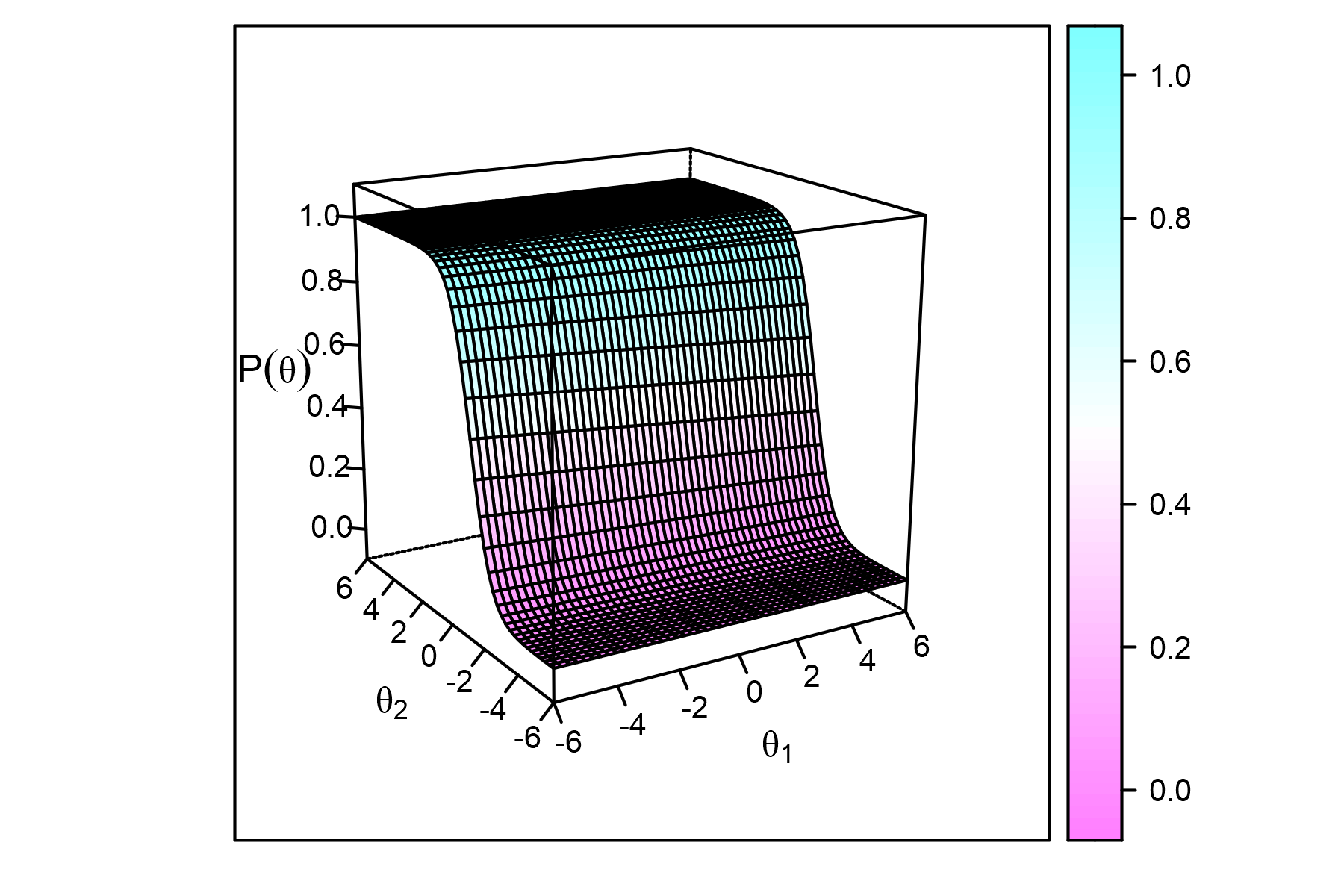
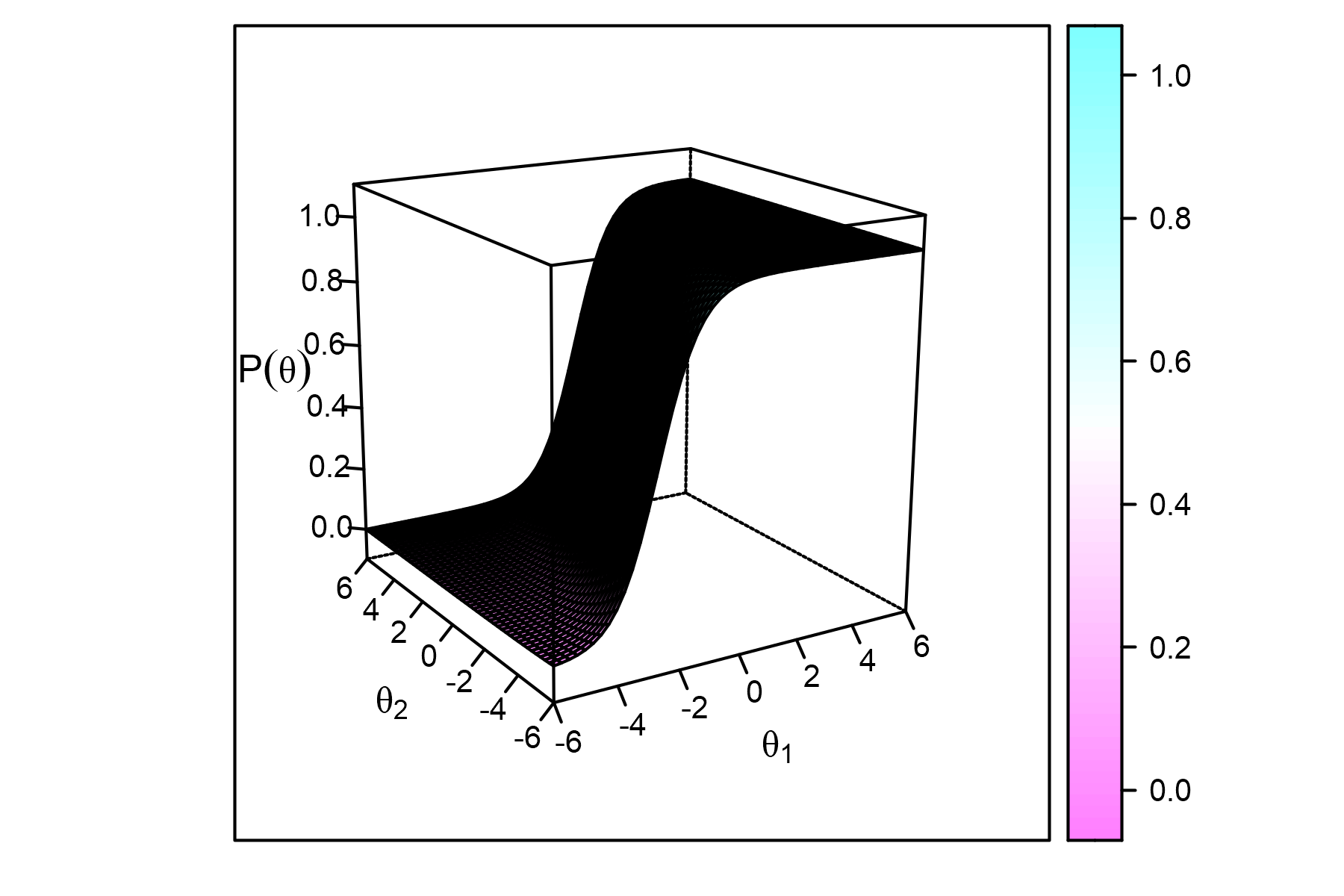
BFI2 dataset.
The two items strongly load on different factors, which is also visible from the surface plots which face different directions (Figure 8.8).
Functions MDIFF() and MDISC() from the mirt package are used to extract multidimensional difficulty and discrimination indices.
MDIFF(m2PL)
##     MDIFF_1
## i1  -1.2465
## i6  -1.2305
## ...
## i4  -0.5545
## ...
MDISC(m2PL)
##     i1     i6    i11    i16    i21    i26    i31    i36    i41
## 1.8548 1.8896 0.5401 2.3346 1.7972 0.9268 2.2508 0.8626 1.4868
##    i46    i51    i56     i4     i9    i14    i19    i24    i29
## 2.1646 1.7246 1.2201 1.6293 1.2734 1.9687 1.3930 1.2216 2.5930
##    i34    i39    i44    i49    i54    i59
## 1.4385 2.3060 1.5733 1.3502 2.3491 2.1542
The results suggest item i29 having the highest overall slope.
Factor scores for both dimensions are extracted using the fscores() function.
head(fscores(m2PL), n = 3)
##           F1      F2
## [1,]  0.0525  1.3830
## [2,] -0.9720  1.2715
## [3,]  1.1962 -2.1297
The first respondent scored 0.05 SD above average on the first (Extraversion) factor, and 1.38 SD above mean on the second (Negative Emotionality) factor.
8.3.2 Multidimensional graded response model
The multidimensional GRM extends the model Equation 8.1 to multiple dimensions. The model assumes \(K_i + 1\) categories \(k = 0, \dots, K_i.\) The cumulative probability of gaining at least \(k\) points, given the respondent’s \(p\) multidimensional latent ability levels \(\boldsymbol{\theta}_p\), is modeled as \[ \pi^{*}_{pik} = \Pr(Y_{pi} \geq k|\boldsymbol{\theta}_p) = \frac{\exp\left(\beta_{0ik} + \boldsymbol{\beta}_{1i} \boldsymbol{\theta}_p\right)}{1 + \exp\left(\beta_{0ik} + \boldsymbol{\beta}_{1i} \boldsymbol{\theta}_p\right)}, \ k = 1, \dots, K_i, \tag{8.13}\]
where \(\boldsymbol{\beta}_{1i}\) are vectors of item-specific slopes and \(\beta_{0ik}\) are ordered category-specific intersections. For the first category \(k = 0\), the cumulative probability is \(\pi^{*}_{pi0} = 1\).
The category probability, i.e., the probability that an item response is exactly \(k\), is \[ \pi_{pik} = \Pr(Y_{pi} = k|\boldsymbol{\theta}_p) = \pi^{*}_{pik} - \pi^{*}_{pi(k + 1)}, \ k = 0, \dots, K_i - 1, \] while for the last category \(k = K_i\) the category probability is equal to the cumulative probability, \(\pi_{piK_i} = \pi^{*}_{piK_i}\), since there is no higher category.
Multidimensional GRM in the mirt. As an example, we fit the two-dimensional GRM Equation 8.13 on the Extraversion and Negative Emotionality items of the BFI2 dataset using the mirt() function from the mirt package. This time, we do not binarize the data, and we use the original ordinal items:
mGRM <- mirt(BFI2en, model = 2, itemtype = "graded")The model parameters are printed with the coef() method.
coef(mGRM, simplify = TRUE)
## $items
##         a1     a2    d1     d2     d3     d4
## i1  -0.125  1.863 4.925  2.293  0.864 -2.174
## i6  -0.187  1.594 4.611  2.090  0.608 -2.067
## ...
## i4   1.747 -0.581 3.453  0.963 -0.578 -3.228
## ...
## i54  1.938 -1.066 2.539  0.179 -1.261 -3.919
## i59  1.973  0.000 3.153  0.435 -0.992 -3.636
##
## $means
## F1 F2
## 0  0
##
## $cov
## F1 F2
## F1  1  0
## F2  0  1
Once more, the first 12 items from the Extraversion domain load strongly on the second factor, with a2 indices further from zero, and the next 12 items from the Negative Emotionality domain load strongly on the first latent factor, having a1 further from zero.
The surface plots are again plotted with the itemplot() function (Figure 8.9).
itemplot(mGRM, item = "i1")
itemplot(mGRM, item = "i4")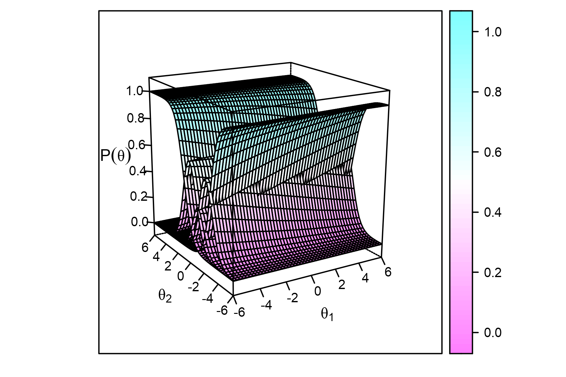
BFI2 item 1.
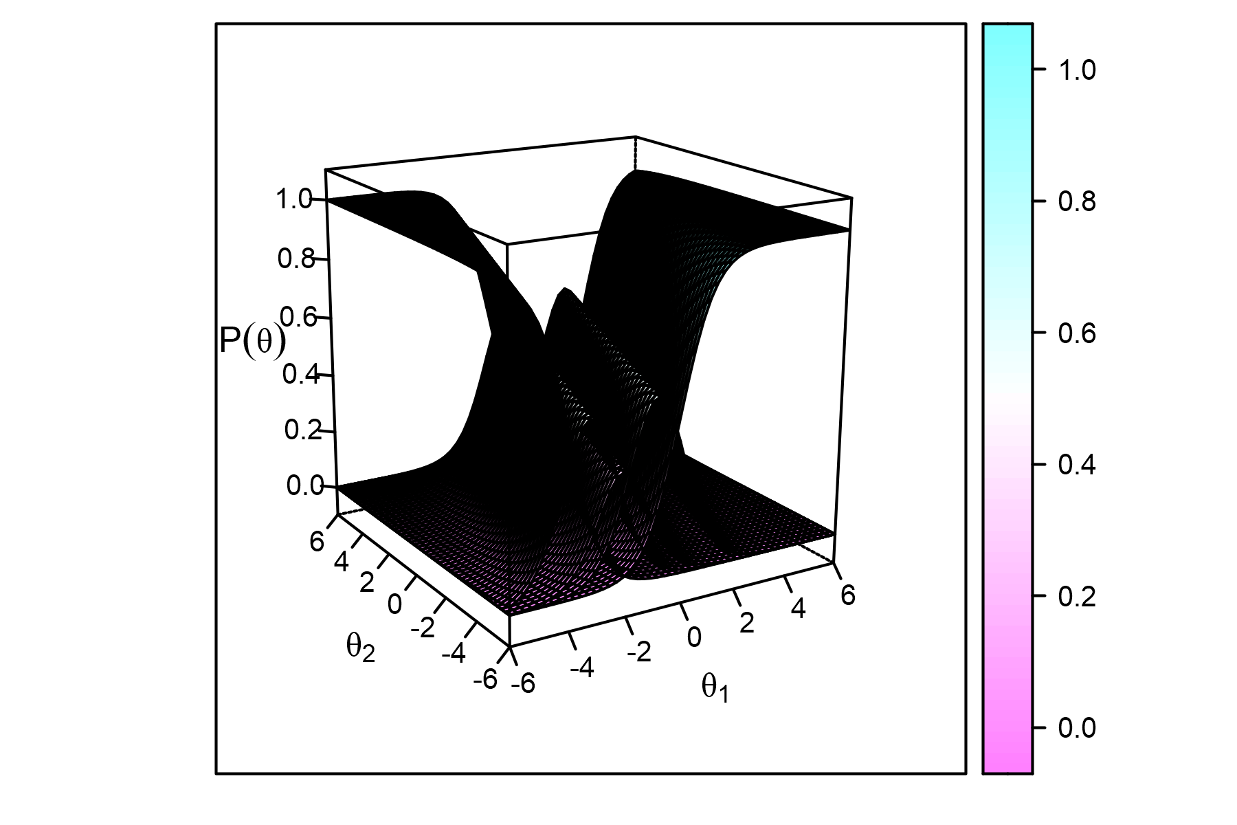
BFI2 item 4.
BFI2 dataset.
As for the two-dimensional 2PL model, the two items from different domains which strongly load on different factors provide the surface plots oriented in opposite directions (Figure 8.9).
The ability estimates, a.k.a. factor scores, are extracted using the fscores() function.
head(fscores(mGRM), n = 3)
##           F1     F2
## [1,]  0.4821  1.274
## [2,] -1.1366  1.160
## [3,]  3.4887 -3.497
Compared to estimates obtained with the 2PL multidimensional IRT model, when the original ordinal items are analyzed, the first respondent is estimated to be 0.48 SD above average on the first (Extraversion) factor and 1.27 SD above mean on the second (Negative Emotionality) factor.
8.3.3 Confirmatory multidimensional IRT models
Confirmatory multidimensional IRT models set further restrictions on some of the model parameters, more specifically, some of the slope parameters in the exploratory multidimensional models, e.g., in the multidimensional 2PL IRT model Equation 8.12 or in the multidimensional IRT GRM Equation 8.13; some of the slopes in vectors \(\boldsymbol{\beta}_{1i}\) are fixed at 0.
Confirmatory multidimensional IRT models in R. As an example, we fit a confirmatory multidimensional GRM Equation 8.13 on the BFI2 dataset. We restrict the first 12 items to load only on the Extraversion factor and the last 12 items to load only on the Negative Emotionality factor. This is done by specifying the factors, here denoted as N and E in the model. We also let the covariance of the two factors be freely estimated by specifying COV = N * E in the model. The model is fitted using the mirt() function from the mirt package.
model_ENirt <- "N = 13-24
                E = 1-12
                COV = N * E"
mGRMc <- mirt(BFI2en, model = model_ENirt, itemtype = "graded")
The model coefficients are displayed with the coef() method:
coef(mGRMc, simplify = TRUE)
## $items
##        a1    a2    d1     d2     d3     d4
## i1  0.000 1.815 4.847  2.264  0.855 -2.141
## i6  0.000 1.668 4.685  2.136  0.626 -2.104
## ...
## i4  1.855 0.000 3.468  0.969 -0.579 -3.242
## ...
## i54 2.164 0.000 2.511  0.187 -1.237 -3.857
## i59 1.679 0.000 2.900  0.405 -0.902 -3.341
##
## $means
## N E
## 0 0
##
## $cov
##        N      E
## N  1.000 -0.366
## E -0.366  1.000
As expected, the first slope parameter a1 (describing loading on the Negative Emotionality factor) is zero in the first 12 items, and the second slope parameter a2 (describing loading on the Extraversion factor) is zero in the last 12 items. The covariance between the two factors is estimated at \(-0.37\).
The surface plots are again plotted with the itemplot() function.
itemplot(mGRMc, item = "i1")
itemplot(mGRMc, item = "i4")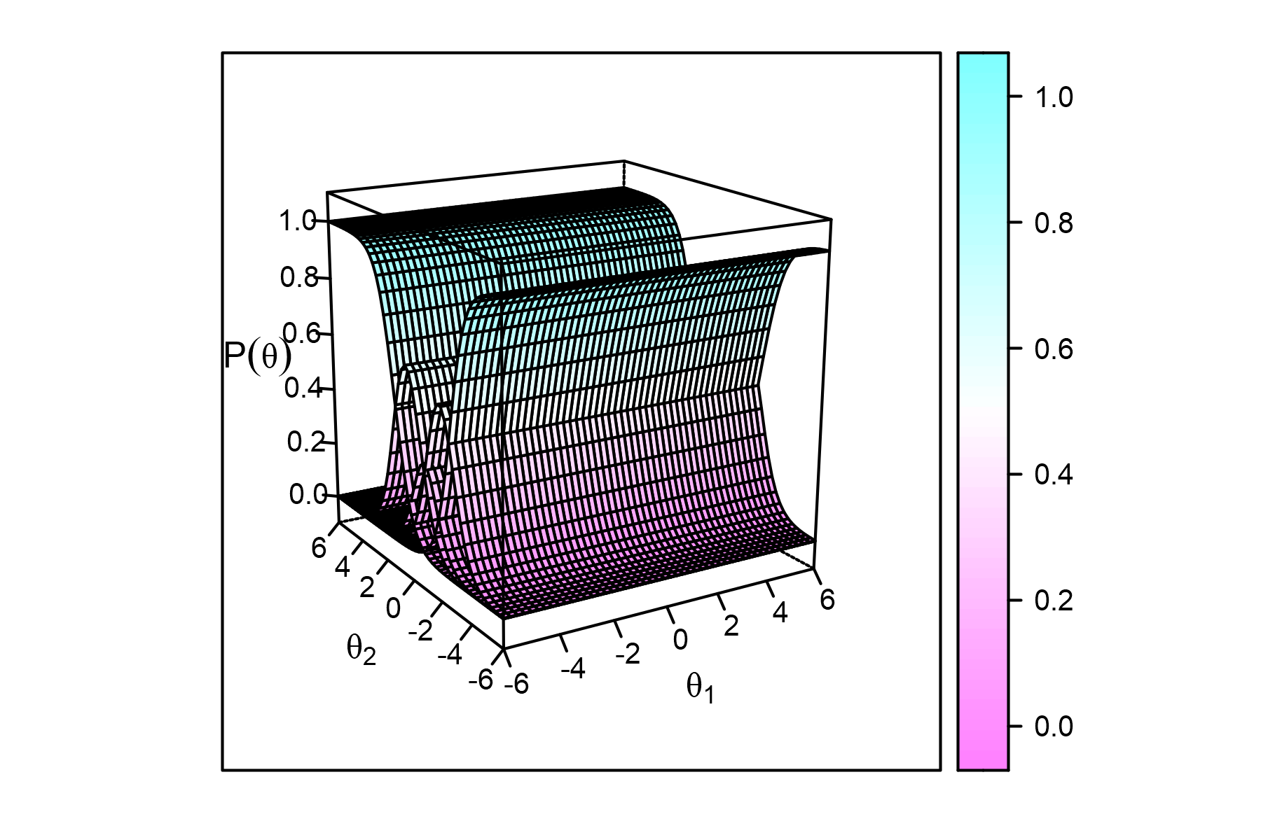
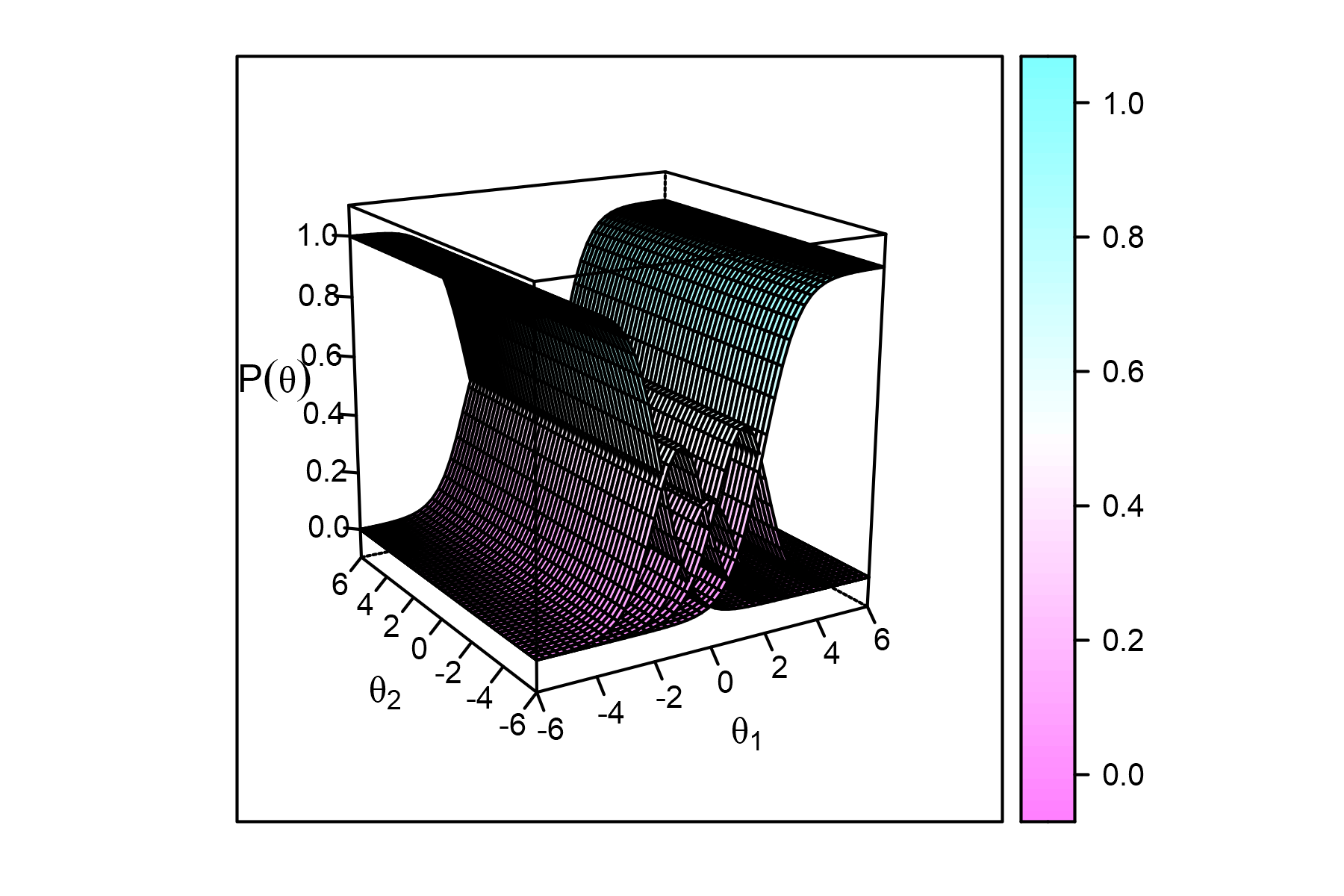
BFI2 dataset.
The two surface plots again face different direction. Compared to previous surface plots, the slices which are given by a fixed level of the N factor (for item 1 “I am someone who is outgoing, sociable”) or of the E factor (for item 4 “I am someone who is relaxed, handles stress well”) would this time create identical IRCs of unidimensional models (Figure 8.10).
To compare the two nested models, i.e., the restricted confirmatory model and the unrestricted exploratory multidimensional GRM Equation 8.13, we can use the LRT Equation 2.29, or information criteria such as AIC Equation 2.30 or BIC Equation 2.31 provided in the anova() method.
 anova(mGRMc, mGRM)
##            AIC    SABIC       HQ      BIC    logLik      X2 df p
## mGRMc 108683.9 108959.9 108928.1 109344.3 -54220.94
## mGRM  107943.5 108269.6 108232.1 108723.9 -53828.74 784.412 22 0
In this case, the information criteria as well as the LRT suggest the unrestricted model fits better, whereas the criteria values are smaller for this model and the p-value is close to 0.
8.4 Estimation in more complex IRT models
8.4.1 Maximum likelihood methods
The three ML estimation methods for binary models, presented in Section 7.3, can be generalized to polytomous items and multidimensional latent traits. In the JML method, to generalize the joint likelihood function Equation 7.8, we use the binary indicators \(y_{pik}\) defined as \(y_{pik} = 1\) when \(y_{pi} = k\), that is, when respondent \(p\) gained \(k\) points in item \(i\), and it is otherwise defined as \(y_{pik} = 0\). The likelihood then has the form \[ L(\boldsymbol{\xi}, \boldsymbol{\theta}) = \Pr(\boldsymbol{Y} = \boldsymbol{y}|\boldsymbol{\theta}, \boldsymbol{\xi}) = \prod_{p = 1}^n \prod_{i = 1}^m \prod_{k = 0}^{K_i} \pi_{pik}^{y_{pik}}, \] where \(\boldsymbol{\xi}\) is a set of item parameters, \(\boldsymbol{\theta}\) is now a vector describing the respondent’s multidimensional latent trait, and \(\pi_{pik}\) is given by an IRT model, now possibly multidimensional and involving polytomous items.
As was already the case in binary IRT models, it is easier to maximize the logarithm of the likelihood function, which now has the form \[ l(\boldsymbol{\xi}, \boldsymbol{\theta}) = \log(L(\boldsymbol{\xi}, \boldsymbol{\theta}))= \sum_{p = 1}^n \sum_{i = 1}^m \sum_{k = 0}^{K_i} y_{pik} \log(\pi_{pik}). \]
The maximization incorporates a calculation of partial derivatives and solving a system of so-called likelihood equations in which derivatives of the log-likelihood function with respect to the estimated parameter are set at equal to zero.
To estimate person abilities with the MML approach, methods presented in Section 7.3.4.1 for binary models can be generalized to polytomous and/or multidimensional models. For a respondent with a given response pattern \(\boldsymbol{y} = (y_{10}, \dots, y_{mK_m})\), the ML estimate of their multidimensional latent trait \(\boldsymbol{\theta}\) can be obtained by maximizing the likelihood function \[ L(\boldsymbol{\xi}, \boldsymbol{\theta}) = \Pr(\boldsymbol{Y} = \boldsymbol{y}|\boldsymbol{\theta}, \boldsymbol{\xi}) = \prod_{i = 1}^m \prod_{k = 0}^{K_i} \pi_{ik}^{y_{ik}}. \] Other methods presented in Section 7.3.4.1 may also be used.
8.4.2 Regularization methods
With a large number of estimated parameters, ML estimation methods may be computationally demanding. To perform regularization and prevent overfitting, the penalty-based methods have been increasingly used (Hastie et al., 2009). The penalty term restricts the parameters; the best known lasso-type penalties shrink some of the parameters towards zero. Penalty-based methods were originally designed for metric variables. They are also recently being implemented in IRT estimation, see Battauz (2020) or Sun et al. (2016).
8.4.3 Bayesian methods with MCMC and MH-RM
For three and more dimensions, the speed of estimation may be increased with the use of the MCMC and the Metropolis-Hastings Robbins-Monroe (MH-RM) algorithm (Cai, 2010). Stochastic approximations, adaptive quadrature, and Laplace approximations are also popular in high dimensional IRT models (Andersson & Xin, 2021; Camilli & Geis, 2019).
8.4.4 Model selection and model fit
The choice between the models should be driven by several aspects. The most important aspect is their underlying data assumptions. Is a single latent trait being modeled, or are multiple latent traits expected? Are the data ordinal with explicit ordering or rather nominal, such as with multiple-choice items? Are we more interested in modeling the ability level needed to provide a response category higher than a certain score (e.g., “disagree” or “mostly disagree” vs. “mostly agree” or “agree”)? If so, models based upon cumulative logits may be more appropriate. Or are we interested in modeling the ability needed to move from one response category to the next one? If this is the case, we may prefer models based on adjacent-categories logit models. The next important aspect is the number of data (i.e., the sample size) available. A lower sample size may force us to use a simpler model even when it does not fully describe the situation.
As was shown throughout this chapter, model selection for nested models can be performed using the LRT Equation 2.29. Competing models may also be compared with the information criteria such as AIC Equation 2.30, BIC Equation 2.31, and their modifications. If the task is to select between the two models of the same number of parameters (e.g., GRM vs. GPCM), we advise not comparing them with information criteria, but rather select the preferred model based upon the type of parameters one wishes to estimate and to interpret.
Model fit may be examined with goodness-of-fit tests and item fit or person fit measures. Fit indices used in FA may also be used considering the earlier described relationship between the IRT and FA models.
8.5 More complex IRT models in interactive application
The section IRT models of the ShinyItemAnalysis application offers fitting the NRM under different parametrizations. The default option is the Bock’s parametrization Equation 8.7. One may, alternatively, use the parametrization from Equation 8.9 proposed by Thissen et al. (2011). The two parametrizations accounting for the correct answer (BL-IS and BL-IRT) are also available. With the BL-IRT parametrization, one can check the graphical interpretation of the estimated parameters (Figure 8.11). The NRM may also be used for ordinal items. In this case, by default, the highest score is considered to be the baseline category.
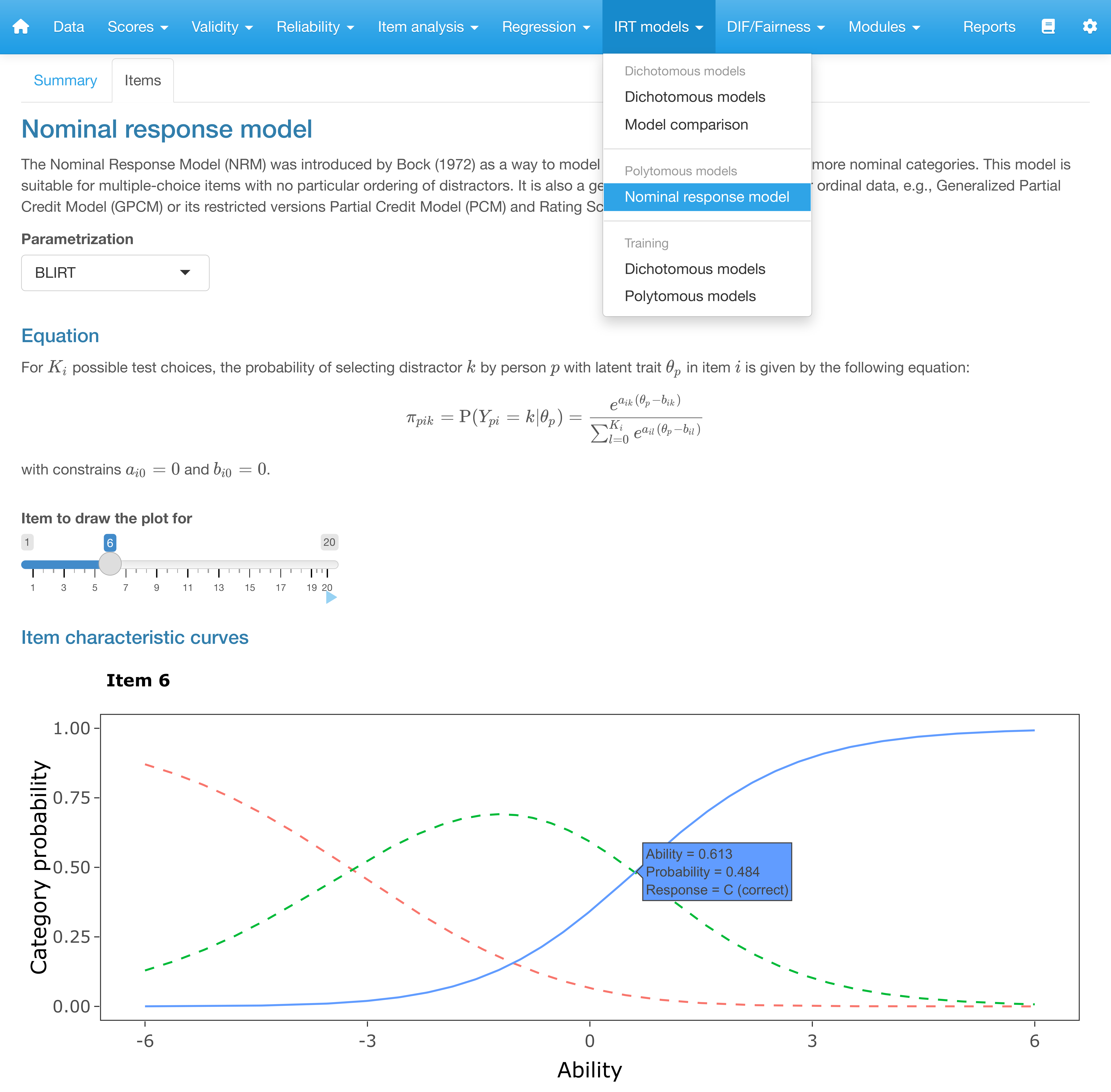
ShinyItemAnalysis.
As for the binary IRT models, the application provides the IICs, together with a table summarizing estimated item parameters, complemented with item fit statistics. A table with estimated respondent abilities is offered for download, and the relationship between standardized total scores and estimated latent abilities (factor scores) is displayed in a scatter plot. A sample R code is provided on the bottom of the page.
An interactive training section is available for additional polytomous IRT models: GRM, (G)PCM, as well as for the NRM.
In the training sections, cumulative probabilities are displayed for the GRM, and IRCs are available for all three models. Additionally, the expected item score is displayed for all of the models. Training sections for the GRM and GPCM also contain interactive exercises where users may check their understanding of the IRT models. Interactive exercises include tasks involving sketching of the ICCs and IICs with given parameters, and questions on the probabilities of correct answers and on the information provided by these items for respondents with certain ability levels.
8.6 Summary
In this chapter, we have presented more complex IRT models, relaxing the earlier assumptions from Chapter 7. We have presented generalizations for polytomous items, ordinal models using the cumulative logits and the adjacent-categories logits, and nominal models involving baseline-category logits for multiple-choice items. We have also discussed multidimensional models which allowed simultaneous estimation of multiple latent traits. The methods were illustrated with practical examples, mostly in the mirt, ltm, and ShinyItemAnalysis packages. The section on estimation discussed the extension of likelihood to polytomous and multidimensional models and further algorithms which may improve upon estimations in these more complex models.