4 Reliability
4.1 Introduction
We have already discussed that measurement error is omnipresent in behavioral research. Typically, we are interested in an applicant’s knowledge, ability, or other trait, but have available for observation and evaluation only the test or interview score. This score may also include measurement errors as a result of fluctuations in the psychological and health state of the applicant, the difficulty of the assigned version of the test, or the leniency of the rater who is grading it.
Natural questions then arise regarding how much information about the true score is indeed contained in the measurement, how strong is the relationship between the true and observed score, and, if being measured repeatedly under the same conditions, how consistent would such repeated measurements be. The answer is provided by various estimates of reliability.
Reliability is an important aspect of measurement mainly because of its relationship to validity. A nice graphical representation of the relationship between reliability and validity is provided in Figure 4.1.
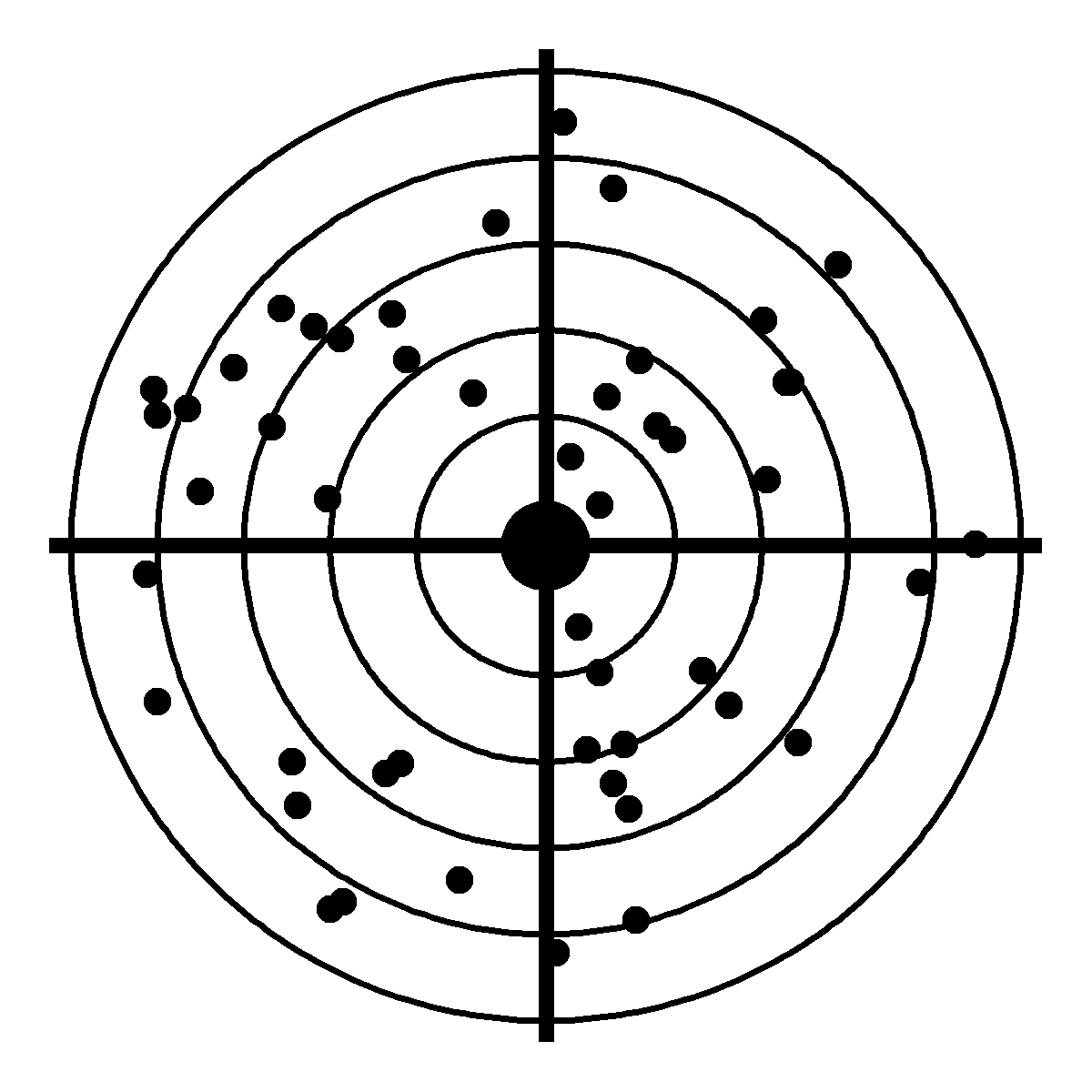
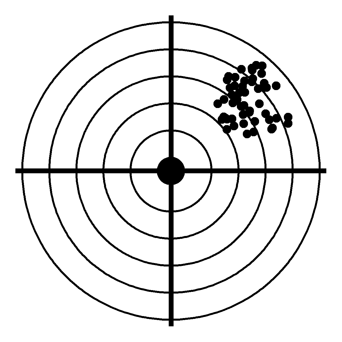

The center of the target represents the trait we want to measure, such as knowledge, ability, anxiety, fatigue, or pain. Shots represent independent measurements of one object. Reliability is then related to variability of the shots, and it is displayed as their mutual closeness, whereas the validity is represented by the overall shots’ closeness to the center. Low reliability always implies low validity: When the variability of the shots is high, we rarely hit the center (Figure 4.1 (a)). On the other hand, high reliability does not ensure high validity: Shots can be very precisely hitting a spot outside of the center (Figure 4.1 (b)). In other words, validity is always bounded by a measurement’s reliability, but reliability itself is not enough to provide a valid measurement. Besides high reliability the measurement has to target the concept being measured in order to provide valid test scores (Figure 4.1 (c)).
In the following sections, we will start with the classical definition of reliability found in CTT, as it was defined and studied by many authors including Spearman (1904) and later Lord & Novick (1968). We will discuss properties of reliability under CTT and discuss the possible ways of increasing reliability. We will then turn to methods for estimation of reliability in Section 4.3, covering approaches based upon correlation coefficients as well as methods based on variance decomposition with the ANOVA method, ML, and Bayesian estimation. More attention will be given to Cronbach’s alpha, a popular estimator of reliability. We will extend the concept of reliability in Section 4.4 devoted to generalizability theory by allowing more sources of error, and we will discuss other reliability estimates in Section 4.5. Section Section 4.6 will present implementations in interactive ShinyItemAnalysis application.
4.2 Formal definition and properties in CTT
Using the notion of CTT, in educational, psychological, and health-related measurement, we are typically interested in the true score, such as the subjects’ ability, knowledge, trait, attitude, pain, fatigue, or quality of life, which are all latent (unobserved). What we actually have available on an educational test, psychological instrument, or health-related questionnaire is only the observed score, contaminated by a measurement error.
4.2.1 Definition of reliability
Let’s assume we have a person’s observed score \(X\) representing their latent ability with their true score \(T\), which is measured with a measurement error of \(e\), so that \[ X = T + e. \tag{4.1}\] We also assume some positive variances of the random variables representing the true score \(\text{Var}(T) = \sigma^2_T\), of the error \(\text{Var}(e) = \sigma^2_e\), and of the observed measurement \(\text{Var}(X) = \sigma^2_X\).
Reliability is then defined as the squared correlation between the true and observed score \[ \text{Rel}(X) = \rho_{X} \coloneqq \text{Cor}^2(T, X). \tag{4.2}\] Theoretical values of reliability belong to the interval \(\rho_X \in \langle 0, 1\rangle\). Low values close to 0 represent a weak alignment between the measurement (observed score) and the corresponding latent variable, thus lower reliability. High values close to 1 mean a closer alignment of the measurement with the latent variable, thus higher reliability.
In a case where the error term is uncorrelated with the true score, i.e., \(\text{Cov}(T, e) = 0\), the squared correlation from Equation 4.2 can be re-expressed as follows \[ \text{Cor}^2(T, X) = \frac{\text{Cov}^2(T, X)}{\text{Var}(T)\text{Var}(X)} = \frac{\text{Cov}^2(T, T + e)}{\text{Var}(T)\text{Var}(X)} = \frac{\text{Var}^2(T) + 0}{\text{Var}(T)\text{Var}(X)} = \frac{\text{Var}(T)}{\text{Var}(X)}. \] The reliability Equation 4.2 can therefore be equivalently defined as the ratio of the true score variance to the total observed variance, \[ \rho_{X} \coloneqq \frac{\sigma^2_T}{\sigma^2_X}, \tag{4.3}\] which may also be re-expressed in analogous forms using \(\sigma^2_X = \sigma^2_T + \sigma^2_e\), \[ \rho_{X} = \frac{\sigma^2_T}{\sigma^2_X} = \frac{\sigma^2_X - \sigma^2_e}{\sigma^2_X} = 1 - \frac{\sigma^2_e}{\sigma^2_X}= \frac{\sigma^2_T}{\sigma^2_T + \sigma^2_e}. \tag{4.4}\] High values close to one represent measurements with a low proportion of error variance, thus high reliability, whereas low values close to zero represent measurements with a high proportion of error variance, thus low reliability.
Note: some authors employ squared correlation from Equation 4.2 to define reliability (Webb et al., 2006) while some prefer a ratio of variances from Equation 4.3. Others directly employ both as equivalent definitions (Mair, 2018; Revelle, 2015), assuming that the error term is uncorrelated with the true score.
4.2.2 Reliability as correlation between measurements
Since the true score \(T\) is not observed, it is not possible to estimate reliability directly from its definition Equation 4.2 or Equation 4.3. Reliability estimation procedures thus typically employ some type of composite or repeated measurements, as we will discuss in more detail in Section 4.3. Here we will discuss some assumptions typically put on the measurements and how they imply that reliability can be understood as a correlation between the two measurements.
Parallel measurements. Let’s assume having two measurements of the same true score, \(X_1 = T + e_1\) and \(X_2 = T + e_2\), which are equally precise, \(\text{Var}(e_1) = \text{Var}(e_2) = \sigma^2_e\), and with uncorrelated errors, \(\text{Cor}(e_1, e_2) = 0\). Such two measurements are called parallel measurements.
Essentially \(\tau\)-equivalent measurements. Two measurements \(X_1 = T_1 + e_1\) and \(X_2 = T_2 + e_2\) with true scores differing by a constant \(T_1 = T_2 + b\), which are equally precise, \(\text{Var}(e_1) = \text{Var}(e_2) = \sigma^2_e\), and with uncorrelated error terms, \(\text{Cor}(e_1, e_2) = 0\), are called essentially \(\tau\)-equivalent measurements.
Note that under the assumption of errors uncorrelated with the true score, \(\text{Cov}(T, e) = 0\), the variance terms of two parallel or essentially \(\tau\)-equivalent measurements are the same, as well as is their reliability \(\text{Rel}(X_1) = \text{Rel}(X_2) = \rho\). From the uncorrelation of the errors of the two measurements, it follows that the correlation between the two measurements is equal to their (common) reliability: \[ \rho_{{X_1, X_2}} = \frac{\text{Cov}(X_1, X_2)}{\sqrt{\text{Var}(X_1)\text{Var}(X_2)}} = \frac{\text{Cov}(T + e_1, T + e_2)}{\sqrt{\text{Var}(T + e_1)\text{Var}(T + e_2)}} = \frac{\sigma^2_T}{\sigma^2_X} = \rho. \tag{4.5}\] This is very practical, as it gives a number of possibilities to easily estimate reliability, as we show more closely in Section 4.3.
While for most of the next sections we will stick with the assumption of at least essential \(\tau\)-equivalence, weakening this assumption may motivate further reliability estimates which will be introduced later in the book. For completeness, we present the nomenclature here:
Weak \(\tau\)-equivalent measurements. Two measurements \(X_1 = T_1 + e_1\) and \(X_2 = T_2 + e_2\) of true scores differing by a constant \(T_1 = T_2 + b\), which are possibly unequally precise with variances \(\text{Var}(e_1)\) and \(\text{Var}(e_2)\), and with uncorrelated error terms, \(\text{Cor}(e_1, e_2) = 0\), are called weakly \(\tau\)-equivalent measurements.
Congeneric measurements. Two measurements of the same true score, although possibly with different slope \(X_1 = \lambda_1 T + e_1\) and \(X_2 = \lambda_2 T + e_2\), and with possibly different error score variances \(\text{Var}(e_1)\), \(\text{Var}(e_2)\), but uncorrelated errors, \(\text{Cor}(e_1, e_2) = 0\) are called congeneric measurements.
4.2.3 Implications of low reliability
Low reliability may have profound implications on assessment, such as less accurate estimates of the true score, wider (less precise) confidence intervals, or attenuated correlations.
Less accurate estimates of the true score. Standard error of measurement can be derived from Equation 4.4: \[ \sigma_e = \sigma_X \sqrt{1 - \rho_{X}}. \tag{4.6}\] Therefore, the lower the reliability \(\rho_{X}\) of the measurement, the higher the standard error of measurement and the less accurate the estimates of the true score will be. With less reliable measurements, we will also get wider confidence intervals for the true scores, and we will need higher number of subjects to demonstrate differences between groups when keeping the same test power.
Attenuation of correlations. As we already pointed out in the Introduction section, reliability limits the predictive validity. Let’s formalize this observation. Predictive validity is often enumerated by correlation between the measurement and a criterion variable. Assuming two imprecise measurements \(X_1 = T_1 + e_1\) and \(X_2 = T_2 + e_2\) of latent variables \(T_1\) and \(T_2\), measured with reliabilities \(\rho_{X_1}\) and \(\rho_{X_2}\), their correlation is attenuated by the square root of the product of their reliabilities: \[ \text{Cor}(X_1, X_2) = \text{Cor}(T_1, T_2)\sqrt{\rho_{X_1}\rho_{X_2}} \leq \text{Cor}(T_1, T_2). \tag{4.7}\] Thus, the correlation we observe is a smaller amount than the correlation between true latent variables. This has negative implications when providing proofs of criterion validity. Correction for attenuation is sometimes implemented to take this fact into account and to enumerate what the expected correlation would be if the measurement was more reliable.
4.2.4 Rules of thumb
Conventional requirements and rules of thumb may vary by the scientific field. For psychological assessment, Cicchetti (1994) provides the following recommendation for classification of reliability values: \[ \rho_{X} \begin{cases} < 0.4 & \text{poor}, \\ \in [0.4, 0.6) & \text{fair}, \\ \in [0.6, 0.75) & \text{good}, \\ \geq 0.75 & \text{excellent}. \end{cases} \] Nunnally & Bernstein (1994) suggested that a reliability of \(\rho_X \geq 0.7\) may suffice in the early stage of instrument development, but in much applied research a reliability of \(0.8\) is not nearly high enough; also see Lance et al. (2006) for discussion on this cutting value. Lee (2012) cites Rust & Golombok (2014) for further discussion about cutting value in different types of assessments: \[ \rho_{X} \begin{cases} \geq .9 & \text{for intelligence tests}, \\ \geq .7 & \text{for personality tests}, \\ \sim .6 & \text{for essay marking}. \end{cases} \] Note, however, that the cutoffs above are rather arbitrary, and therefore should be used with discretion. Also, the uncertainty in reliability estimates (e.g., in the form of a confidence interval) should be taken into account when interpreting results.
4.2.5 Reliability of composites
One way of increasing reliability is by using an average or sum of multiple measurements. Composite measurements are common in educational tests, scales, or questionnaires, where the instrument is composed of a higher number of items with the goal of providing multiple converging pieces of information. Similarly, when rating applicants or grant proposals, often times more than one rater is involved and an average rating is used for making decisions.
Let’s assume having \(m > 1\) parallel or essentially \(\tau\)-equivalent measurements \(X_1, \dots, X_m\) of the same true score \(T\). Then the composite measurement \(X = \sum_{i = 1}^{m} X_i\) has the reliability \[ \rho_{X} = \rho_{m} = \frac{\text{Var}(m T)}{\text{Var}(\sum_{i = 1}^m X_i)} = \frac{\text{Var}(m T)}{\text{Var}(m T + \sum_{i = 1}^m e_i)} = \frac{m^2 \sigma^2_T}{m^2 \sigma^2_T + m \sigma^2_e} = \frac{\sigma^2_T}{\sigma^2_T + \frac{\sigma^2_e}{m}}. \tag{4.8}\]
Note that the reliability of the composite measurement \(\rho_{m}\), where \(m > 1\), is higher than the reliability of its component \(\rho_{1}\) due to a lower measurement error \(\frac{\sigma^2_e}{m}\). The same relationship also holds for the average rating \(\bar{X} = \frac{1}{m}\sum_{i = 1}^{m} X_i\). Formula Equation 4.8 implies that by adding enough parallel items or raters we may, at least theoretically, increase the reliability as close to 1 as we desire.
4.2.5.1 Spearman-Brown prophecy formula
The Spearman-Brown prophecy formula enumerates the relationship between the reliability of a composite measurement \(\rho_{m}\) and the reliability of its component \(\rho_{1}\) (Brown, 1910; Spearman, 1910): \[ \rho_{m} = \frac{m\rho_{1}}{1 + (m - 1)\rho_{1}}. \tag{4.9}\] One way to derive the Spearman-Brown formula is to use the definition of \(\rho_{1}\) in Equation 4.3 and the formula Equation 4.8 for \(\rho_{m}\).
More generally, the Spearman-Brown formula can also provide a relationship between the reliability of shorter and longer tests: Assume a test composed of \(m_1\) parallel or essentially \(\tau\)-equivalent measurements and its prolonged or shortened version composed of \(m_2\) such measurements. Then the relationship between reliabilities of their total scores \(X_{(1)} = \sum_{i = 1}^{m_1} X_i\), and \(X_{(2)} = \sum_{i = 1}^{m_2} X_i\) is \[ \rho_{m_2} = \frac{\frac{m_2}{m_1} \rho_{m_1}}{1 + (\frac{m_2}{m_1} - 1)\rho_{m_1}}. \tag{4.10}\]
Finally, the Spearman-Brown formula can also be used to calculate the number of items needed when the goal is to reach a certain level of reliability. This is a very practical use of the formula, which may serve for decisions on test length. To calculate the number of necessary items to obtain specific reliability, we first derive a ratio of the test length \(m = m_2/m_1\) and then multiply the original number of items by this ratio. From formula Equation 4.10, it follows that \[ m_2 = m_1 \frac{\rho_{m_2} (1 - \rho_{m_1})}{\rho_{m_1} (1 - \rho_{m_2})}, \tag{4.11}\] therefore, the number of necessary items is given as the next highest integer of \(m_2\).
Spearman-Brown formula in R. Calculations with the Spearman-Brown formula are straightforward and easy to implement in R. Consider for example a test with a reliability of 0.75 composed of 20 items (20 parallel measurements). We want to estimate the reliability if the test were prolonged by 10 equally precise items measuring the same construct. We first calculate ratio \(m\) of test lengths and then implement formula Equation 4.10.
rho_original <- 0.75 # reliability of original data
items_original <- 20 # number of items in original data
items_new <- 30 # number of items in new data
(m <- items_new / items_original) # ratio of tests lengths
## [1] 1.5
m * rho_original / (1 + (m - 1) * rho_original) # new reliability
## [1] 0.8182
The reliability of the prolonged test would be 0.82. The same result is provided by the SBrel() function of the psychometric package. Argument Nlength specifies how many times the original test is prolonged (or shortened); argument rxx specifies the original reliability.
library(psychometric)
SBrel(Nlength = m, rxx = rho_original)
## [1] 0.8182
The second question is how many items are needed if we want to obtain a composite measurement with a reliability of 0.85. We implement the formula Equation 4.11 to calculate the desired ratio of test lengths \(m\), and we then multiply this ratio by the original test length, while also rounding to the closest higher or equal integer with the ceiling() function.
rho_new <- 0.85
(m <- rho_new * (1 - rho_original) / (rho_original * (1 - rho_new)))
## [1] 1.8889
ceiling(m * items_original)
## [1] 38
To get a reliability of 0.85, we would need 38 items. The same result can be obtained with the SBlength() function of the psychometric package. Argument rxxp specifies the desired reliability; rxx contains the original reliability. The result is the ratio \(m\) which again needs to be multiplied by the original test length and rounded to obtain the desired test length.
(m <- SBlength(rxxp = rho_new, rxx = rho_original))
## [1] 1.8889
ceiling(m * items_original)
## [1] 38
As before, we conclude that to get a reliability of 0.85 we would need 38 items.
We now compute how many items are needed if a reliability of 0.7 was sufficient.
rho_new <- 0.7
(m <- rho_new * (1 - rho_original) / (rho_original * (1 - rho_new)))
## [1] 0.7778
ceiling(m * items_original)
## [1] 16
The same result can be obtained with the psychometric package:
(m <- SBlength(rxxp = rho_new, rxx = rho_original))
## [1] 0.7778
ceiling(m * items_original) # new test length
## [1] 16
Based on the prophecy formula, 16 items would be enough to obtain a composite measurement with reliability of 0.7.
4.2.6 Increasing reliability
There are several approaches available for solving a problem of low reliability. As implied from the Spearman-Brown formula, one can increase the reliability by adding more items to a composite measurement or by adding more raters while making decisions on the basis of average rating. The assumption of parallel (essentially \(\tau\)-equivalent) measurements means that new items/raters have to measure the same construct with equal precision.
In the case of multiple raters, reliability may be increased by providing more precise instructions (e.g., in a detailed rating rubric), rater training, and/or by requiring a formal certification.
Reliability may also be increased by item or rater weighting. The weighted average is then used as a composite score instead of the average or the total score. Optimal weights maximizing the reliability can be derived in different scenarios (Mosier, 1943). Caution is needed, because implementing the weights maximizing the reliability may decrease the validity of the measurement.
Another way of increasing reliability is to inspect the functioning of each single item or rater (see Chapter 5). Inconsistent or badly functioning items need to be reworded, deleted and/or replaced. However, such processes may be quite costly; thus it is important to be sure the reliability is estimated properly: Overestimation may result in adopting an unreliable instrument, while underestimation may imply an (unnecessary) instrument revision, which is also undesirable.
4.3 Estimation of reliability
The simplest estimates of reliability are correlation coefficients between two observed total scores in multiple measurements. Cronbach’s alpha, a popular reliability estimator, is related to average inter-item correlation.
4.3.1 Reliability estimation with correlation coefficients
Reliability estimates based upon multiple administrations make use of Equation 4.5 and are simple correlation coefficients between two observed total scores. Depending on the type of replication, different types of reliability can be distinguished. One type is a test-retest reliability which uses the same instrument twice. Another method uses parallel forms of the instrument. Finally, a test can be divided into parts (such as halves of items), and correlation of the subscores, corrected for the test length, can provide yet another reliability estimate, as we describe below.
4.3.1.1 Test-retest reliability
For the test-retest reliability estimate, exactly the same instrument is given to the respondents. To prevent the respondents from remembering the items, it is recommended to perform the second measurement after a certain period of time, e.g., 3 months. In the case of educational tests, respondents should not get any training between the two administrations; however, even with this restriction, some learning usually occurs. The correlation coefficient between total scores from the two administrations is then used as an estimate of reliability, usually denoted as coefficient of stability.
Test-retest reliability in R. The example is presented with the HCI, the HCItestretest dataset. We first divide the dataset to test and retest data.
data(HCItestretest, package = "ShinyItemAnalysis")
HCI_test <- HCItestretest[HCItestretest$test == "test", ]
HCI_retest  <- HCItestretest[HCItestretest$test == "retest", ]
The scatterplot of test and retest total scores suggests positive correlation between the test and the retest score (Figure 4.2, see Supplementary R code).
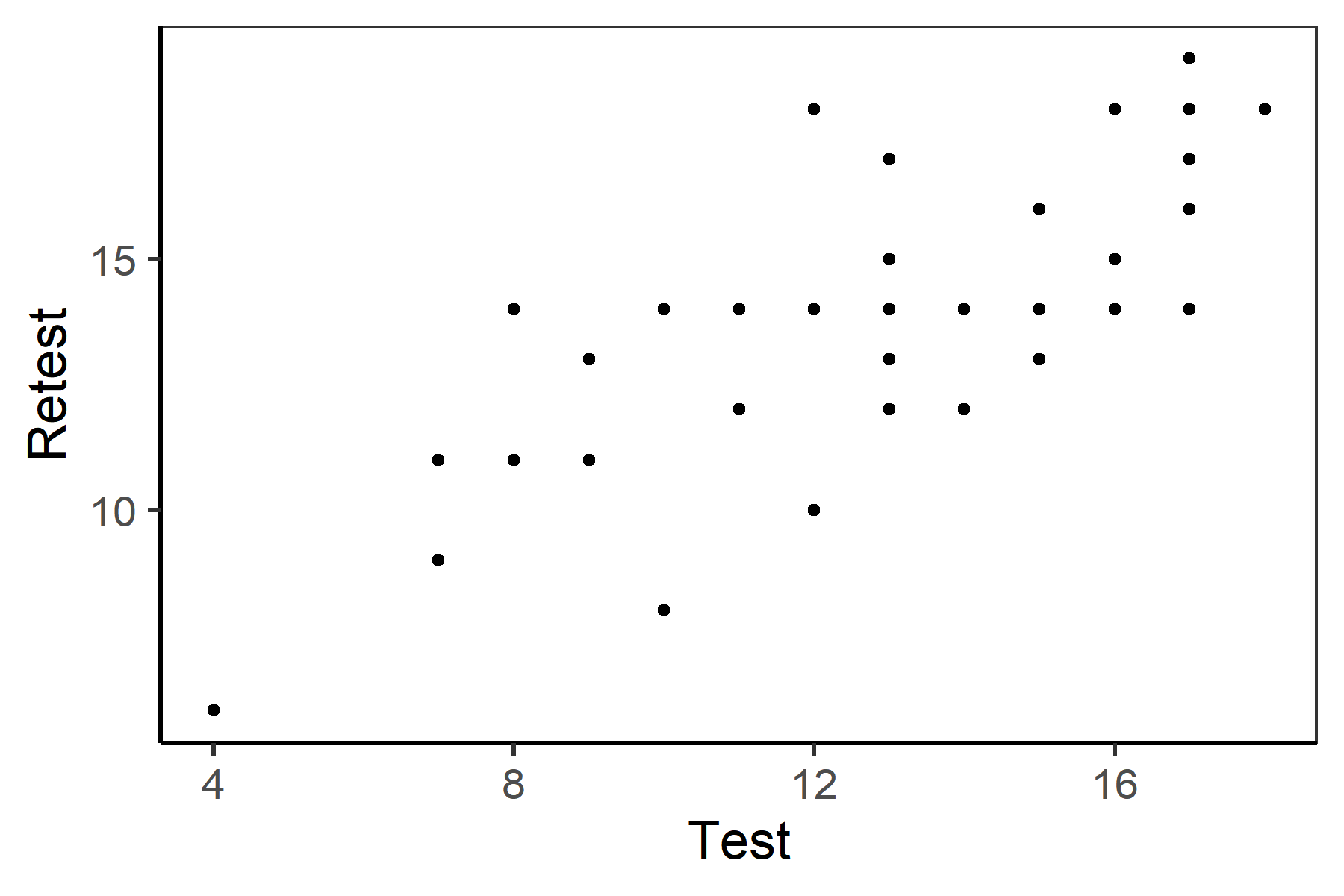
HCItestretest dataset.
The cor.test() function is used here to provide an estimate of correlation coefficient between the test and the retest total scores, and the confidence interval, and to test whether the correlation significantly differs from zero.
cor.test(HCI_test$total, HCI_retest$total)
## Pearson's product-moment correlation
##
## data:  HCI_test$total and HCI_retest$total
## t = 7.914, df = 43, p-value = 6.278e-10
## alternative hypothesis: true correlation is not equal to 0
## 95 percent confidence interval:
##  0.6156 0.8675
## sample estimates:
##       cor
## 0.7700
Pearson’s correlation coefficient of 0.77 with a 95% confidence interval of \((0.62, 0.87)\) is significantly nonzero (\(t\) = 7.91, df = 43, p-value < 0.001); using Cicchetti’s rule of thumb, the test-retest reliability of the HCItestretest dataset can be categorized from good to excellent.
4.3.1.2 Parallel forms
Another approach for multiple administrations is to assign two versions of the same instrument to the same group of respondents. The two versions should contain items with the same content and properties, which in an ideal case are parallel forms. Again, the correlation coefficient between total scores from the two forms is then used as an estimate of reliability; usually denoted as coefficient of equivalence.
4.3.1.3 Split-half coefficient
Multiple administrations may be costly and cause an additional burden to tested subjects. Therefore, estimates of reliability often use data from a single administration only. In such cases, reliability estimates are often based upon the fact that the instrument is composed of multiple items. These estimates are often denoted as coefficients of internal consistency.
Split-half coefficients make use of splitting the test into two halves and calculating subscores, \(X^*_1\) and \(X^*_2\), i.e., the total scores which are based only upon items in the first and the second subsets. Correlation between the two subscores \(\text{Cor}(X^*_1, X^*_2)\) is a reliability estimate for a test of half length. The reliability estimate of the original length is then obtained by applying the Spearman-Brown formula Equation 4.9 with \(m = 2\): \[ \rho_X = \frac{2 \cdot \text{Cor}(X^*_1, X^*_2)}{1 + \text{Cor}(X^*_1, X^*_2)}. \tag{4.12}\] Various split-half coefficients are obtained depending upon how the test is divided into the two halves.
First-second split-half approach takes the first half of the items and correlates the subscore based upon these items with the subscore based on the second half of the items. A reliability estimate based upon this approach may be underestimating the true reliability: In the case of lengthy tests, respondents may be more tired when answering the second half of the items. In tests with increasing difficulty of items, the correlation between the subscores from the first and second half will typically also be lower than for other split-half methods.
As an alternative, the even-odd approach includes even items into the first subset and odd items into the second one. A random approach consists of performing a random split of items. The resulting estimate is usually slightly different for each random draw.
One can also consider the best split-half or the worst split-half, or even analyze the distribution of all possible reliability estimates based upon different splits, which may give an idea of how much the different split-half estimates can vary. While the calculation of such estimates may be time-consuming for longer instruments, the software implementations can make approximations by taking only a defined number of randomly selected split-halves to calculate the minimum or maximum value.
Another approach to consider is the average split-half of all possible split-half coefficients. Again, a defined number of randomly selected split halves can be used to estimate the average split-half coefficient in the case of longer instruments, if calculations based upon all possible splits would be time-consuming.
Split-half coefficient in R. Demonstration is presented with the HCI dataset, which comprises 20 items.
data(HCI, package = "ShinyItemAnalysis")
HCI_items <- HCI[, 1:20]
We first compute the first-second split-half. The data is divided into the first and the second half. The partial total scores are computed, and the correlation between the two partial total scores is calculated. The Spearman-Brown formula Equation 4.12 is then applied to obtain the estimate of reliability.
df1 <- HCI_items[, 1:10]; df2 <- HCI_items[, 11:20]
ts1 <- rowSums(df1); ts2 <- rowSums(df2)
cor_x <- cor(ts1, ts2)
2 * cor_x / (1 + cor_x)
## [1] 0.6966
Using the first-second split-half, the reliability is estimated at 0.70.
Next, we apply the even-odd split-half approach. The seq() function is used to select the odd and the even item numbers.
df1 <- HCI_items[, seq(1, 20, 2)]; df2 <- HCI_items[, seq(2, 20, 2)]
ts1 <- rowSums(df1); ts2 <- rowSums(df2)
cor_x <- cor(ts1, ts2)
2 * cor_x / (1 + cor_x)
## [1] 0.7415
The reliability estimate obtained in this way was considerably higher (\(0.74\)) than the first-second split-half coefficient (\(0.69\)).
Further, we apply a random split-half approach. We use the sample() function to randomly select 10 from 20 items and the setdiff() function to select the remaining 10 items. The set.seed() function is used for reproducibility.
set.seed(123)
samp <- sample(1:20, 10)
df1 <- HCI_items[, samp]; df2 <- HCI_items[, setdiff(1:20, samp)]
ts1 <- rowSums(df1); ts2 <- rowSums(df2)
cor_x <- cor(ts1, ts2)
2 * cor_x / (1 + cor_x)
## [1] 0.7386
The reliability estimate obtained by this random split was \(0.74;\) this estimate was similar to the one obtained with the even-odd approach.
4.3.2 Cronbach’s alpha
Cronbach’s alpha (Cronbach, 1951) is probably the most popular measure of internal consistency, most likely for its simplicity. It takes into account item variances and variance of the total scores, which are easy to estimate. However, as we will show, it can also be expressed as a function of the average inter-item correlation. It also has a nice conceptual explanation in the ANOVA framework, which we will discuss more closely in Section 4.3.2.2.
For an instrument with \(m\) items where \(X = \sum_{i = 1}^m X_i\) is the total score, \(\sigma^2_X\) its variance, and \(\sigma^2_{X_i}\) variances of the items, Cronbach’s alpha is defined as \[ \alpha = \frac{m}{m - 1}\left(1 - \frac{\sum_{i = 1}^m \sigma^2_{X_i}}{\sigma^2_X}\right). \tag{4.13}\]
Cronbach’s alpha is based upon the idea of splitting the test into individual items, which are considered, conceptually, to be parallel or at least essentially \(\tau\)-equivalent measurements. Under these assumptions, the Cronbach’s alpha is equal to the reliability of a composite measurement Equation 4.8. In a general case and when errors are uncorrelated, alpha is a lower bound of the reliability \(\alpha\leq\rho_{_X}\) (Novick & Lewis, 1967). In the case of correlated errors, alpha can be either lower or greater than the reliability (Green & Hershberger, 2000).
The sample estimate of Equation 4.13 is \[ \hat{\alpha} = \frac{m}{m - 1} \left(1 - \frac{\sum_{i = 1}^m s_{ii}}{\sum_{i = 1}^m\sum_{j = 1}^m s_{ij}}\right), \tag{4.14}\] where \(s_{ij}\) are terms of the sample variance/covariance matrix \(\mathbb{S}\): \[ s_{ij} = \frac{1}{n - 1} \sum_{p = 1}^n(X_{pi} - \bar{X}_{\bullet i})(X_{pj} - \bar{X}_{\bullet j}), \] with \(\bar{X}_{\bullet i} = \frac{1}{n}\sum_{p = 1}^n X_{pi}\). The last term in Equation 4.14 is a fraction with the total sample variance in the denominator and the sum of sample item variances, i.e., the sum of the main diagonal terms (the trace) of the sample variance/covariance matrix in the numerator.
Cronbach’s alpha in R. Cronbach’s alpha can be easily estimated by plugging directly into the formula Equation 4.13 the sample counterparts of the total score variance \(\sigma^2_X\) and item variances \(\sigma^2_{X_i}\). In the example below, we will again consider the 20-item HCI dataset:
m <- ncol(HCI_items) # number of items
var(HCI$total) # sample variance of total scores
## [1] 13.2473
item_vars <- sapply(HCI_items, var) # item sample variances
m / (m - 1) * (1 - (sum(item_vars)) / var(HCI$total))
## [1] 0.7155
The Cronbach’s alpha is estimated at 0.72.
The formula Equation 4.14 provides a more elegant implementation in R. We first estimate the variance/covariance matrix with the var() function and then calculate the trace as the sum of its diagonal terms calculated with the diag() function,
VC <- var(HCI_items)
(m / (m - 1)) * (1 - sum(diag(VC)) / sum(VC))
## [1] 0.7155
which again gives an estimate of 0.72.
Implementation of the Cronbach’s alpha estimate is also provided with the alpha() functions in both the psych package and in the psychometric package:
psych::alpha(HCI_items)$total[1]
## raw_alpha
## 0.7155
psychometric::alpha(HCI_items)
## [1] 0.7155
The resulting estimates of \(0.72\) from both alpha() functions are in an exact agreement with our previous calculations. Besides an estimate of Cronbach’s alpha based on the raw data, the psych package also provides its version based on standardized data employing correlations rather than covariances, and other useful indices (see Supplementary R code).
4.3.2.1 Cronbach’s alpha and inter-item correlations
Cronbach’s alpha can also be expressed as a function of average inter-item covariance \(\bar{c} = \frac{\sum_{i \neq j} \text{Cov}(X_i, X_j)}{m (m - 1)}\) and of average item variance \(\bar{v} = \frac{\sum_{i = 1}^m \sigma^2_{X_i}}{m}\):
\[ \alpha = \frac{m}{m - 1}\left(1 - \frac{\sum_{i = 1}^m \sigma^2_{X_i}}{\sigma^2_X}\right) = \frac{m}{m - 1} \frac{\sum_{i \neq j} \text{Cov}(X_i, X_j)}{\sum_{i = 1}^m \sigma^2_{X_i} + \sum_{i \neq j} \text{Cov}(X_i, X_j) } = \frac{m \bar{c}}{\bar{v} + (m - 1)\bar{c}}. \tag{4.15}\] Note that with parallel items of variance equal to one, formula Equation 4.15 becomes the Spearman-Brown prophecy formula Equation 4.9.
Cronbach’s alpha and inter-item correlations in R. Implementation of estimation of Cronbach’s alpha with formula Equation 4.15 into R is demonstrated using the HCI dataset,
(c_bar <- sum(sapply(1:m, function(i) {
  sum(cov(HCI_items[, i], HCI_items[, -i]))
})) / (m * (m - 1)))
## [1] 0.0237
(v_bar <- sum(item_vars) / m)
## [1] 0.2122
m * c_bar / (v_bar + (m - 1) * c_bar)
## [1] 0.7155
which once more leads to the same estimate of reliability of 0.72.
4.3.2.2 Cronbach’s alpha and ANOVA
Cronbach’s alpha can also be explained through ANOVA. In this framework, the item data are viewed as repeated measurements and are analyzed with a random-effect model, in which the true score differences of the respondents are viewed as a random effect. The variance of the random effect is compared to the residual variance, and Cronbach’s alpha is then estimated as their ratio. We will present the idea first with a simple one-way model, and then extend it to a two-way model.
One-way random-effect model. The one-way random-effect model is the simplest random-effect model for repeated measurements. Conceptually it is very close to ITT Equation 4.1: \[ X_{pi} = \mu + T_p + e_{pi}, \tag{4.16}\] where \(\mu\) is the overall mean (an intercept for a fixed effect), \(T_p\) is a random effect of person \(p\), and \(e_{pi}\) is a random error term. The random effects \(T_p\) and \(e_{pi}\) are further assumed to be normally distributed, \(T_p \sim \mathcal{N}(0, \sigma^2_P)\) and \(e_{pi} \sim \mathcal{N}(0, \sigma^2_e)\). The variance of the random person effect \(\sigma^2_P\) is the true-score variance, the variance of the residual \(\sigma^2_e\) is the error variance, and the total variance \(\sigma^2_X = \sigma^2_P + \sigma^2_e\) is the sum of the two.
The single-rating reliability is then defined by the same formula as Equation 4.4: \[ \hat{\rho}_1 = \frac{\hat{\sigma}^2_P}{\hat{\sigma}^2_P + \hat{\sigma}^2_e}, \tag{4.17}\] and the multiple-rating (\(m\)-item composite) reliability estimator corresponds to the estimate in Equation 4.8: \[ \hat{\rho}_m = \frac{\hat{\sigma}^2_P}{\hat{\sigma}^2_P + \hat{\sigma}^2_e / m}. \tag{4.18}\]
The simplest approach for estimation of variance components in the random-effect model Equation 4.16 is using the ANOVA method. See Table 4.1 for an overview of typical one-way ANOVA notation.
| Source | \(df\) | \(SS\) | \(MS\) |
|---|---|---|---|
| Person | \(n - 1\) | \(SS_P = m \sum_{p = 1}^n (\bar{X}_{p\bullet} - \bar{X}_{\bullet\bullet})^2\) | \(MS_P = \frac{SS_P}{n - 1}\) |
| Residual | \(n(m-1)\) | \(SS_e = \sum_{p = 1}^n \sum_{i = 1}^m (X_{pi} - \bar{X}_{p\bullet})^2\) | \(MS_e = \frac{SS_e}{n(m-1)}\) |
| Total | \(nm - 1\) | \(SS_T = \sum_{p=1}^n \sum_{i=1}^m (X_{pi} - \bar{X}_{\bullet\bullet})^2\) |
\(\bar{X}_{p\bullet}\) represents an average measurement of person \(p\) and \(\bar{X}_{\bullet\bullet}\) a grand mean. The \(F\) statistic is calculated as a ratio of the two mean squares \(F = MS_P / MS_e\), and can further be used for inference, such as construction of the confidence interval.
In the balanced design, the ANOVA estimates of variance components of model Equation 4.16 are obtained from the expected mean squares: \[ \hat{\sigma}^2_e = MS_e \text{ and } \hat{\sigma}^2_P = \frac{MS_P - MS_e}{m}. \] This leads to the following estimator of single-rating reliability (the intraclass correlation coefficient, ICC): \[ \hat{\rho}_1 = \frac{MS_P - MS_e}{MS_P + (m - 1) MS_e}, \] and the composite measurement reliability (Cronbach’s alpha): \[ \hat{\alpha} = \hat{\rho}_m = 1 - \frac{MS_e}{MS_P} = 1 - \frac{1}{F}. \] The confidence interval for Cronbach’s alpha then follows from the confidence interval for the \(F\) statistic: \[ \hat{\alpha} \in \left\langle 1 - \frac{F_{1-\gamma/2}(n - 1, (m - 1)(n - 1))}{F};\ 1 - \frac{F_{\gamma/2}(n - 1, (m - 1)(n - 1))}{F} \right\rangle, \tag{4.19}\] where \(F_{\gamma}(n - 1,(m - 1)(n - 1))\) denotes the \(\gamma\) quantile of a Fisher-Snedecor distribution with \(n - 1\) and \((m - 1)(n - 1)\) degrees of freedom.
Two-way models. Another extension of the one-way model is the two-way random effect model: \[ X_{pi} = \mu + T_p + B_i + e_{pi}, \tag{4.20}\] with an additional random effect for item (or rater) \(B_i \sim \mathcal{N}(0, \sigma^2_I)\). In this model, each rating contains not only the random true score difference of each respondent and random noise, but also the item (or rater) random effect. \(\sigma^2_I\) is the item variance (including e.g., the item difficulty), and \(\sigma^2_e\) is the residual variance (now representing person-item interaction variance in addition to random noise).
A two-way mixed-effect model, \[ X_{pi} = \mu + T_p + b_i + e_{pi}, \tag{4.21}\] represents the situation when items are fixed (not random), with item effect denoted by \(b_i\).
While the one-way ANOVA provides the estimate of single-rating reliability for the AIBS dataset, the two-way ANOVA gives the estimate of Cronbach’s alpha for the HCI (or HCIlong) data.
One-way ANOVA in R. We first demonstrate the one-way ANOVA approach on the AIBS dataset. The dataset describes a study evaluating 72 research project proposals in the field of behavioral sciences. Each proposal is rated on scientific merit on a 1–5 scale by 3 reviewers. An excerpt is displayed:
data(AIBS, package = "ShinyItemAnalysis")
head(AIBS[, c("ID", "Score")], n = 9)
##     ID Score
## 1 ID1     3
## 2 ID1     4
## 3 ID1     5
## 4 ID2     2
## 5 ID2     3
## 6 ID2     4
## 7 ID3     2
## 8 ID3     2
## 9 ID3     2
The dataset is already in a long format. The numbers of respondents (proposals) and items (raters) are:
(n <- length(unique(AIBS$ID)))
## [1] 72
(m <- nrow(AIBS) / n)
## [1] 3
To perform the one-way random-effect ANOVA Equation 4.16, we can use the aov() function in base R:
model <- aov(Score ~ Error(ID), data = AIBS)
summary(model)
## Error: ID
##           Df Sum Sq Mean Sq F value Pr(>F)
## Residuals 71  50.39  0.7097
##
## Error: Within
##            Df Sum Sq Mean Sq F value Pr(>F)
## Residuals 144  57.56  0.3997
The table provides the sums of squares and the mean squares, which are estimates of expected mean squares. Using these values, we estimate the variance between persons (among raters/proposals) \(\hat{\sigma}^2_P\) and the error variance \(\hat{\sigma}^2_e\):
(MSe <- 0.3997) # or equivalently: summary(model)[["Error: Within"]][[1]]["Residuals", "Mean Sq"]
## [1] 0.3997
(MSP <- 0.7097) # or equivalently: summary(model)[["Error: ID"]][[1]]["Residuals", "Mean Sq"]
## [1] 0.7097
Using formula for ANOVA estimates:
(sigma2P <- (MSP - MSe) / m) # true score variance estimate
## [1] 0.1033
(sigma2e <- MSe) # error variance estimate
## [1] 0.3997
Single-rating reliability:
sigma2P / (sigma2P + sigma2e) # single-rating reliability
## [1] 0.2055
Multiple-rating (composite) reliability:
sigma2P / (sigma2P + sigma2e / m) # composite reliability for m raters
## [1] 0.4369
The single-rating reliability is estimated at 0.21. The 3-rater composite reliability is estimated at 0.44.
Two-way ANOVA for Cronbach’s alpha in R. To demonstrate estimation of Cronbach’s alpha with the two-way ANOVA approach, we use the HCIlong dataset, the long format variant of the HCI dataset.
data(HCIlong, package = "ShinyItemAnalysis")
head(HCIlong, n = 3)
##     id item rating
## 1 ID1    1      1
## 2 ID1    2      1
## 3 ID1    3      1
The numbers of respondents and items:
(n <- length(unique(HCIlong$id)))
## [1] 651
(m <- length(unique(HCIlong$item)))
## [1] 20
Mean squares from the two-way ANOVA can be directly plugged into a formula for estimation of person variance, and then used to calculate the Cronbach’s alpha estimate:
model2 <- aov(rating ~ id + item, data = HCIlong)
(MSP <- summary(model2)[[1]]["id", "Mean Sq"])
## [1] 0.2122
(MSe <- summary(model2)[[1]]["Residuals", "Mean Sq"])
## [1] 0.1885
(FA <- MSP / MSe)
## [1] 1.1260
1 - 1 / FA
## [1] 0.1119(sigma2P <- (MSP - MSe) / m)
## [1] 0.0012
sigma2P / (sigma2P + MSe / m)
## [1] 0.1119The \(F\) statistic is used for a derivation of the two-sided 95% confidence interval Equation 4.19. The qf() function is used to compute the quantiles of a Fisher-Snedecor distribution.
gamma <- 0.05 # significance level
# lower bound in 95% two-sided confidence interval
1 - qf(1 - gamma / 2, n - 1, (m - 1) * (n - 1)) / FA
## [1] 0.6828
# upper bound in 95% two-sided confidence interval
1 - qf(gamma / 2, n - 1, (m - 1) * (n - 1)) / FA
## [1] 0.7462
The resulting reliability estimate is again \(0.72\). The confidence interval of this estimate is \((0.68, 0.75)\) which is in exact agreement with the results from the psychometric package.
a <- psychometric::alpha(HCI_items)
psychometric::alpha.CI(a, N = nrow(HCI_items), k = ncol(HCI_items), level = 0.95)
##      LCL  ALPHA    UCL
## 1 0.6828 0.7155 0.7462
And the confidence interval is also approximately in agreement with the results from the psych package:
psych::alpha(HCI_items)$feldt
## 95% confidence boundaries (Feldt)
## lower alpha upper
##  0.68  0.72  0.75
4.3.3 Further estimation of variance components
4.3.3.1 Maximum likelihood
The ML estimation method makes use of the assumption for the underlying probability of the data, in our case, the normal distribution to specify the likelihood function, which is the probability density function given the data \(\boldsymbol{x}\): \[ L(\mu, \mathbb{V}| \boldsymbol{x}) = f(\boldsymbol{x}; \mu, \mathbb{V}), \] with \(\mathbb{V}\) being the variance matrix. The ML estimates of the parameters (\(\mu, \sigma^2_P, \sigma^2_e\)) are then gathered as parameters for which the likelihood is maximal given the data \(\boldsymbol{x}\).
We consider the one-way random effect model Equation 4.16 for simplicity. Under the model, the vector of ratings has a multivariate normal distribution, \[ \boldsymbol{x} \sim \mathcal{N}(\mu\boldsymbol{1}, \mathbb{V}). \] Note that the variance matrix \(\mathbb{V}\) is not a diagonal, but rather a block-diagonal matrix, given that two ratings of the same respondent \(p\) are correlated \[ \text{Var}(x_{pi})= \sigma^2_P + \sigma^2_e, \quad \text{Cov}(x_{pi}, x_{p'i'}) = \begin{cases} \sigma^2_P & \text{for } p = p', \\ 0 & \text{for } p \neq p'. \end{cases} \] The likelihood function is given by the probability density function of the multivariate normal distribution: \[ L(\mu, \mathbb{V} | \boldsymbol{x}) = \frac{\exp[-\frac{1}{2}(\boldsymbol{x} - \mu\boldsymbol{1})' \mathbb{V}^{-1} (\boldsymbol{x} - \mu\boldsymbol{1})]}{(2 \pi)^{\frac{nm}{2}} |\mathbb{V}|^{\frac{1}{2}}}. \] Considering the form of the variance matrix and using matrix algebra, for the balanced design this simplifies to \[ L(\mu, \sigma_P^2, \sigma_e^2| \boldsymbol{x})= \frac{\exp\left[-\frac{1}{2} \left( \frac{SS_e}{\sigma_e^2} + \frac{SS_P + mn (\bar{x}_{\bullet\bullet} - \mu)}{m \sigma_P^2 + \sigma_e^2} \right)\right]}{ (2 \pi)^{\frac{nm}{2}}\sigma^{n(m - 1)} (m \sigma_P^2 + \sigma_e^2)^{\frac{n}{2}}}, \tag{4.22}\] where \(SS_P\) and \(SS_e\) are the sums of the squared deviations between and within respondents.
The ML estimates are found as parameters maximizing the likelihood function Equation 4.22, given the data \(\boldsymbol{x}\). This is equivalent to maximizing the log-likelihood, which is more tractable, since the original likelihood contains the multiplication of very small numbers. The ML estimates are then solutions to the likelihood equations, i.e., the equations in which the partial derivatives (with respect to given parameters) of the log-likelihood are set at zero.
In the simple balanced case of the one-way random effect model Equation 4.16, the likelihood equations can be solved explicitly (see, for example, Searle et al., 2009, p. 80), and yield the following ML estimators for the variance components: \[ \begin{aligned} \hat{\sigma}_e^2 =&\ MS_e \ \text{and} \ \hat{\sigma}_P^2 = \frac{\left(1 - \frac{1}{n}\right) MS_P - MS_e}{m}, &\text{when} \; \left(1 - \frac{1}{n}\right) MS_P \geq MS_e, \\ \hat{\sigma}_e^2 =&\ \frac{SS_P + SS_e}{n m} \ \text{and} \ \hat{\sigma}_P^2 = 0, &\text{when} \; \left(1 - \frac{1}{n}\right) MS_P < MS_e. \end{aligned} \] Note that whenever \(\left(1 -\frac{1}{n}\right) MS_P < MS_e\), we always get a zero estimate of reliability.
For more complicated designs, such as unbalanced designs with a different number of raters per respondent, or designs with more sources of error, the closed forms are typically not available, and the maximization is performed with the use of a numerical algorithm.
Reliability with ML estimate of variance components in R. We fit the one-way random-effect model Equation 4.16 on the AIBS dataset with the lmer() function of the lme4 package. The notation (1 | ID) is used to annotate random effect. We enforce the ML algorithm with an argument REML = FALSE.
library(lme4)
model1_ML <- lmer(Score ~ 1 + (1|ID), data = AIBS, REML = FALSE)
The estimates of variance components are then obtained with the VarCorr() function of the same package:
as.data.frame(VarCorr(model1_ML))
##        grp        var1 var2   vcov  sdcor
## 1       ID (Intercept) <NA> 0.2311 0.4807
## 2 Residual        <NA> <NA> 0.4003 0.6327
In the output, the vcov column contains the variance/covariance components of model effects, while sdcor corresponds to their square root. As expected, the ML estimate of 0.24 for the true-score variance is very similar to the estimate obtained from the ANOVA method, and the estimate of 0.40 for the residual variance is identical to the ANOVA estimate from Section 4.3.2.2.
Next, the variance component estimates are extracted:
(sigma2P_ML <- as.numeric(VarCorr(model1_ML)))
## [1] 0.2311
(sigma2e_ML <- sigma(model1_ML)^2)
## [1] 0.4003
and used for estimation of single-rating reliability:
sigma2P_ML / (sigma2P_ML + sigma2e_ML)
## [1] 0.3660
and for estimation of multiple-rating reliability:
sigma2P_ML / (sigma2P_ML + sigma2e_ML / m)
## [1] 0.6340
The reliability estimate of 0.37 for a single rating, and of 0.63 for a composite rating based on the average of 3 raters, are very similar to those obtained from the ANOVA method.
4.3.3.2 Restricted maximum likelihood
The restricted (or residual) maximum likelihood method is an adaptation in which the marginal likelihood function is maximized with respect to variance components \((\sigma^2_P, \sigma^2_e),\) while the third parameter \(\mu\) is integrated out of the likelihood function: \[ L(\sigma^2_P, \sigma^2_e | \boldsymbol{x}) = \int L(\mu, \sigma_P^2, \sigma_e^2| \boldsymbol{x}) \text{d}\mu. \]
In the simple balanced case of the one-way random effect model Equation 4.16, the restricted likelihood is easily derived and the likelihood equations can be solved explicitly yielding the following REML estimators for variance components: \[ \begin{aligned} \hat{\sigma}_e^2 =&\ MS_e &\text{and} \ \ \hat{\sigma}_P^2 =&\ \frac{MS_P - MS_e}{m}, & \quad \text{when} \;\quad MS_P \geq MS_e, \\ \hat{\sigma}_e^2 =&\ \frac{SS_P + SS_e}{n m - 1} &\text{and} \ \ \hat{\sigma}_P^2 =&\ 0, & \quad \text{when} \;\quad MS_P < MS_e. \end{aligned} \] Note that when \(MS_P < MS_e\), we always get a zero estimate of reliability. When \(MS_P > MS_e\), the REML estimators of variance components in the balanced one-way random effect model are identical to ANOVA estimators; thus the reliability estimators are also the same.
Restricted maximum likelihood estimate in R. We again illustrate a computation on the AIBS dataset with the one-way random-effect model Equation 4.16. In the lmer() function of the lme4 package, the REML algorithm is the default option. Argument REML = TRUE can be specified, but is not necessary. We use the VarCorr() function to obtain estimates of variance components.
model1_REML <- lmer(Score ~ 1 + (1|ID), data = AIBS, REML = TRUE)
as.data.frame(VarCorr(model1_REML))
#        grp        var1 var2   vcov  sdcor
# 1       ID (Intercept) <NA> 0.2362 0.4860
# 2 Residual        <NA> <NA> 0.4003 0.6327
As expected, the REML estimates are identical to ANOVA estimates from Section 4.3.2.2. The differences between ML and REML estimates of variance \(\hat{\sigma}^2_P\) are negligible with this high number of respondents \(n\). Thus also the resulting reliability estimate differs only slightly (see Supplementary R code).
Next, we illustrate an estimation of Cronbach’s alpha with REML for the HCIlong dataset. We fit the two-way random effect model Equation 4.20 using the lmer() function, and we extract the estimates of the variance components with the VarCorr() function of the lme4 package.
model2_REML <- lmer(rating ~ (1 | id) + (1 | item), data = HCIlong)
(VC <- as.data.frame(VarCorr(model2_REML)))
##        grp        var1 var2   vcov  sdcor
## 1       id (Intercept) <NA> 0.0237 0.1539
## 2     item (Intercept) <NA> 0.0270 0.1643
## 3 Residual        <NA> <NA> 0.1885 0.4341
The estimate of Cronbach’s alpha is obtained by plugging in the REML estimates of respondent variance and residual variance into Equation 4.18:
(sigma2P_HCI <- VC[VC$grp == "id", "vcov"])
## [1] 0.0237
(sigma2e_HCI <- VC[VC$grp == "Residual", "vcov"])
## [1] 0.1885
sigma2P_HCI / (sigma2P_HCI + sigma2e_HCI / m)
## [1] 0.7155
The estimate of person variance of 0.02, residual variance of 0.19, and estimate of Cronbach’s alpha of 0.72 are again identical to those obtained with the ANOVA method from Section 4.3.2.2.
4.3.3.3 Bootstrap confidence intervals
The calculation of confidence intervals of reliability estimates based on ML is not straightforward in more complex designs. One option in such situations is to use bootstrap (see, for example, Efron & Tibshirani, 1994). In each run, the bootstrap algorithm re-samples the data and creates a new sample, upon which the model is fitted and variance terms for person, item, and residual variance are estimated. The distribution of these variance terms and their functions (such as reliability estimates) can then be further analyzed using these bootstrapped samples.
Bootstrap in R. We demonstrate the calculation of confidence interval for reliability estimate with Cronbach’s alpha. We use the model Equation 4.21 fitted as model2_REML in the previous section for the HCIlong dataset. In the lme4 package, the bootstrap method is implemented within the bootMer() function. Argument FUN specifies the function of the model to be saved in each re-sampling step; here we save the elements of the variance/covariance matrix estimated with the VarCorr() function. The number of simulation runs is set to 100, which provides relatively stable results in a reasonable time; a higher number such as 1,000 can be used for production.
boot <- bootMer(model2_REML, nsim = 100, seed = 543,
                FUN = function(mm) unlist(as.data.frame(VarCorr(mm))["vcov"]))
The estimates of variance components obtained from each re-sample are saved as individual rows of the boot$t matrix:
bootVars <- as.data.frame(boot$t)
colnames(bootVars) <- VC[, "grp"]
head(bootVars, n = 2)
##        id    item Residual
## 1 0.02382 0.01229   0.1883
## 2 0.02069 0.01420   0.1893
From the first re-sample, the respondent variance is estimated at 0.02, the item variance is estimated at 0.01, and the residual variance at 0.19. Estimates are very similar with the second re-sample.
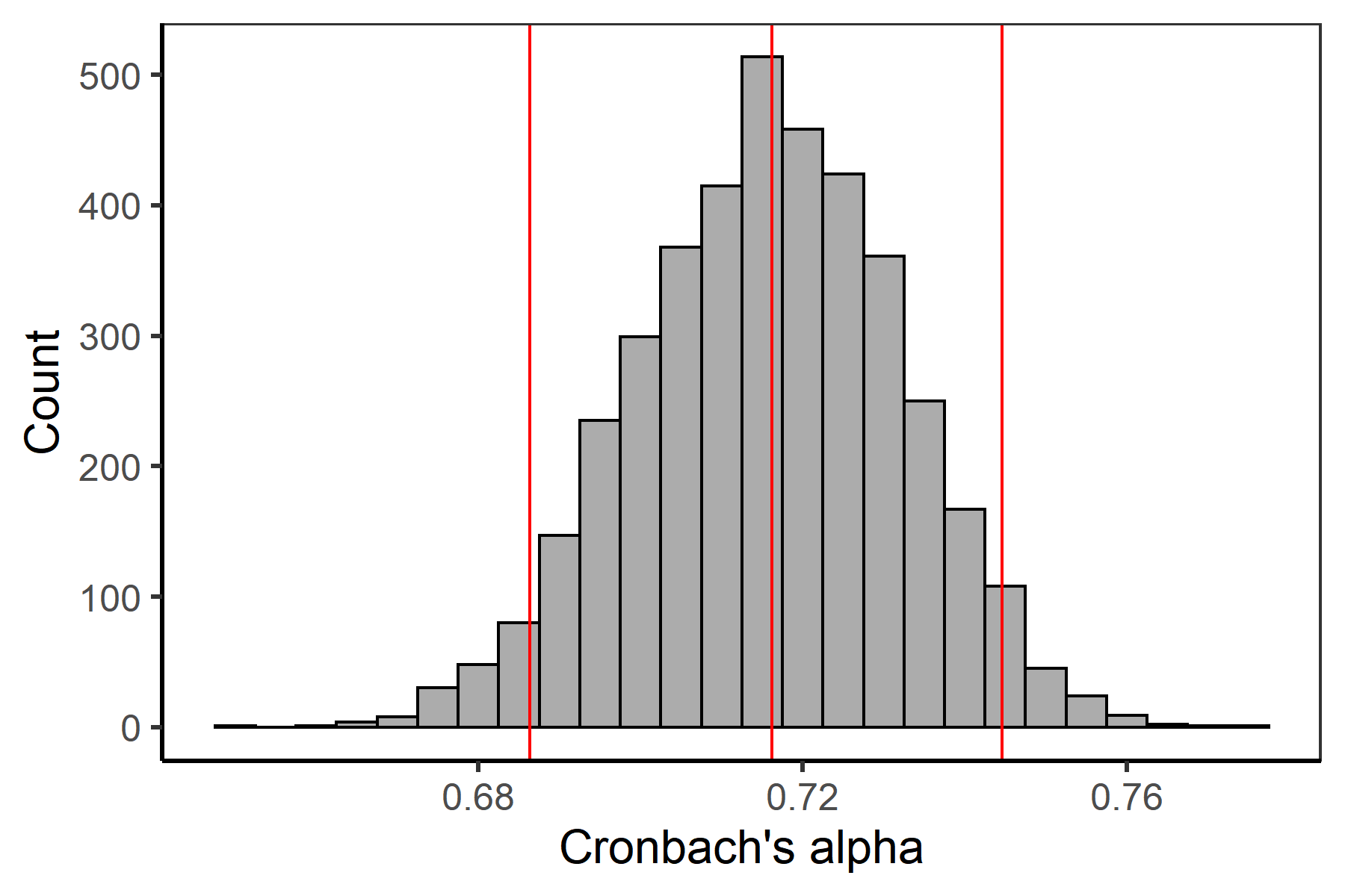
Subsequently, the vectors of estimated variance terms can be combined into a vector of bootstrapped reliability estimates. Distribution of these reliability estimates can be analyzed, e.g., with a histogram (Figure 4.3, see Supplementary R code).
bootAlphaCR <- bootVars[, "id"] / (bootVars[, "id"] + bootVars[, "Residual"] / m)The lower and upper boundaries of the \(95\%\) bootstrapped confidence interval for Cronbach’s alpha are calculated as the \(2.5^{\text{th}}\) and \(97.5^{\text{th}}\) quantiles:
quantile(bootAlphaCR, 0.025)
##      2.5%
##    0.6819
quantile(bootAlphaCR, 0.975)
##     97.5%
##    0.7406
The resulting bootstrapped confidence interval boundaries of \((0.68, 0.74)\) are very similar to those obtained using the \(F\) statistic in Equation 4.18.
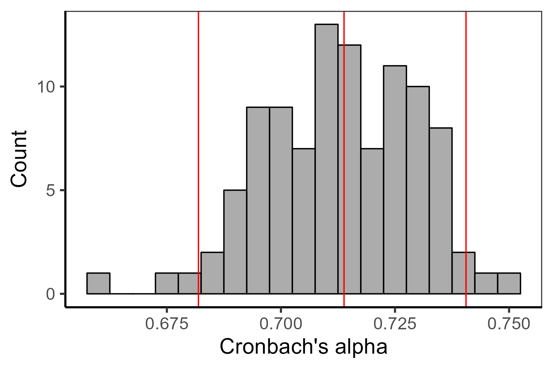
HCI dataset.
4.3.3.4 Bayesian estimation
Contrary to the ML, the Bayesian estimation can avoid the zero estimates by setting assumptions on prior distribution \(p(\sigma^2_P, \sigma^2_e)\). The typical choices of prior distribution for the variance components are the inverse gamma, the half-normal, or the half-student \(t\) distribution. The posterior density \[ p(\sigma^2_P, \sigma^2_e | \boldsymbol{x}) = \frac{f(\boldsymbol{x} | \sigma^2_P, \sigma^2_e) p(\sigma^2_P, \sigma^2_e)}{\int f(\boldsymbol{x} | \sigma^2_P, \sigma^2_e) p(\sigma_P, \sigma_e) \text{d}\sigma_P\text{d}\sigma_e} \] is then enumerated and the Bayesian estimates of \(\sigma^2_P\) and \(\sigma^2_e\) are found as the mean or mode value of this posterior density, accordingly.
Bayesian estimation in R. In R, the package brms1 uses Stan2 software to fit Bayesian models with MCMC. The advantage is that the brms uses the same syntax as the lme4 package. The main brm() function uses a half-\(t\) distribution with 3 degrees of freedom and a scaling parameter of 2.5 as a default option. We demonstrate the estimation of Cronbach’s alpha by fitting the two-way mixed effect model on the HCIlong dataset:
library(brms)
set.seed(1234)
fitB <- brm(rating ~ (1 | id) + (1 | item), data = HCIlong)
The output contains a table of estimated parameters for each generated sample:
results <- as.data.frame(fitB)
head(results[, 1:4], n = 3)
##   b_Intercept sd_item__Intercept sd_id__Intercept  sigma
## 1      0.5501             0.2249           0.1563 0.4412
## 2      0.5880             0.1492           0.1517 0.4307
## 3      0.5827             0.1444           0.1470 0.4295
The Cronbach’s alpha for each generated sample is obtained by plugging the estimates of variance components into the formula Equation 4.14:
alphaCR <- results[, "sd_id__Intercept"]^2 /
  (results[, "sd_id__Intercept"]^2 + results[, "sigma"]^2 / m)
Next, the median and the lower and upper bound of the 95% credible interval are computed using the quantile() function.
quantile(alphaCR, 0.5)
##    50%
## 0.7156
quantile(alphaCR, 0.025)
##   2.5%
## 0.6814
quantile(alphaCR, 0.975)
##  97.5%
## 0.7455
The estimated Cronbach’s posterior median alpha is \(0.72,\) with the 95% uncertainty interval of \((0.68, 0.75)\). The distribution of the estimates together with the median and credible interval is displayed in Figure 4.4 (see Supplementary R code).
HCI dataset.
To conclude, we have presented alternative and more recent approaches to the estimation of reliability, namely the ML and REML, the bootstrap, as well as the Bayesian approach. For the simplest cases, such as balanced one-way and two-way designs, we have shown that the resulting estimates are either identical or almost identical to those obtained by the ANOVA method. The advantage of these methods is in their flexibility when more complex designs are being analyzed.
4.4 More sources of error and G-theory
The concept of reliability can be extended in several ways to accommodate more complex designs. Perhaps the best known extension is the generalizability theory (G-theory) which we will discuss here. The G-theory was introduced by Cronbach et al. (1963) and further refined in Cronbach et al. (1972); see also Brennan (1992). The G-theory allows for more sources of error in Equation 4.1. The main aim is to enumerate variances in all sources of error that are controllable, and to propose more precise or efficient designs.
Calculations with the G-theory were originally based on the ANOVA approach, and consisted of enumeration of mean squares and deriving the reliability estimates using their ratios, similar to Equation 4.17 and Equation 4.18. This may become tricky in more complex designs, with multiple sources of error, and structure other than the fully crossed one. For this reason, when more complex designs are implemented, the effects are often treated as random and their variance is estimated in the framework of random effect models with estimating techniques, such as ML, REML, or Bayesian methods; see Section 4.3.3.
Additional terminology may be helpful before exploring formal derivation and examples. The multiple sources of error (usually termed as effects in statistics) are here termed as facets. Besides items or raters, other examples of facets can be schools, districts, measurement occasions, or trials, to name a few. The combination of facets is termed as conditions. Note that respondents are not sources of error, and are therefore not facets, but objects of measurement. While test or questionnaire respondents are typical objects of measurement, in some cases the objects of measurement can be project proposals (which get rated on a number of criteria by several raters), journal articles (rated by peer-reviewers), or institutions (whose quality is being assessed). The true score from Equation 4.1 in G-theory is termed universe score, and it is assumed to be the mean value of the universe of all possible test realizations on the object of measurement.
The G-theory comprises two parts. First, in the generalizability study (G-study), all possible sources of error are identified, and the variance components are estimated and enumerated as ratios of the total variance. The second part is the dependability study (D-study), which uses the information from the G-study to enumerate reliability indices in different designs. These may involve a different number of facet levels or their combinations. For example, in a study involving items and raters, one may be interested in reliability estimates for cases of 5, 10, and 20 items rated by 1, 2, or 3 raters, which yields 9 combinations. In this aspect, the D-study provides a generalization of the Spearman-Brown formula Equation 4.10.
The G-study and D-study are defined by their number of facets and by their design. The simplest case is a one-facet study. An example of a one-facet study is a study in which all persons are given the same set of items; such a study is termed crossed (and denoted as a \(p \times i\) study). Another example is a study in which the items are nested within persons (denoted as \(i:p\)). Similarly, a two-facet study may involve items and raters as sources of error. These may be fully crossed with persons (\(p \times i \times r)\) or partially nested in different ways. While the G-study should preferably involve crossed designs whenever possible to avoid the confounding of effects, the D-study, on the other hand, may use nested designs for convenience.
What primarily drives the D-study is how we plan to use the test scores. If the test scores are used to make relative decisions (e.g., selecting the top fifth of all applicants), the relative error variance \(\sigma^2_{\text{rel}}\) is estimated, and the reliability of the scores is summarized with the generalizability coefficient \[ \rho^2 = \frac{\sigma^2_P}{\sigma^2_P + \sigma^2_{\text{rel}}}. \tag{4.23}\] If, on the other hand, the test scores are used to make absolute decisions (such as passing all students above a certain level of ability), the absolute error variance \(\sigma^2_{\text{abs}}\) is estimated and the dependability coefficient is used: \[ \phi = \frac{\sigma^2_P}{\sigma^2_P + \sigma^2_{\text{abs}}}. \tag{4.24}\] The key part is thus expression of the relative error variance \(\sigma^2_{\text{rel}}\) and the absolute error variance \(\sigma^2_{\text{abs}}\), which differs under different designs.
4.4.1 A one-facet study
In a one-facet study, respondents are fully crossed with items. In other words, all respondents are assigned the same set of items. If the items are considered to be a random sample within the universe of possible items, this situation corresponds to a two-way random effect model Equation 4.20.
As part of the D-study, the ratios of variances are enumerated by dividing each variance term (\(\sigma^2_P\) for person, \(\sigma^2_I\) for item, and \(\sigma^2_e\) for residual) by the total variance (\(\sigma^2_{\text{total}} = \sigma^2_P + \sigma^2_I + \sigma^2_e\)). When considering composite rating, such as the average score: \[ \bar{X}_{p \bullet} = \frac{1}{m}\sum_{i = 1}^{m} X_{pi} = \mu + T_p + \frac{1}{m}\sum_{i = 1}^{m} B_i + \frac{1}{m}\sum_{i = 1}^{m} e_{pi}, \] the variance of the average item effect is smaller, \(\sigma^2_I / m\), and so is the residual variance, \(\sigma^2_e / m\).
Dependability coefficient. To enumerate the dependability coefficient, we need to calculate the absolute error variance. For single scores, the absolute error is simply the difference between a person’s observed and universe scores, in this case \(X_{pi} - \mu - T_p\). The variance of the absolute error is thusly the sum of all variance components except the one for the persons: \[ \sigma^2_{\text{abs}} = \sigma^2_I + \sigma^2_e. \] For composite measurement based on \(m\) items, the absolute error is \(\bar{X}_{p \bullet} - \mu - T_p\), and the variance of the absolute error is \[ \sigma^2_{\text{abs}} = \frac{\sigma^2_I}{m} + \frac{\sigma^2_e}{m}. \tag{4.25}\]
The square root of the absolute error variance \(\sigma_{\text{abs}}\) is the absolute standard error of variance and can be used for construction of a confidence interval for observed item scores.
The dependability coefficient Equation 4.24, which describes reliability of the \(m\)-item instrument related to absolute decisions, is then equal to the percentage of the observed total variance of the composite score which can be attributed to respondents.
Generalizability coefficient. The generalizability coefficient is related to relative decisions and involves their relative error variance. Relative error is the difference between a person’s observed deviation score and the universe score, in the case of a composite measurement enumerated as \(\bar{X}_{p \bullet} - \mu - T_p - \frac{1}{m}\sum_{i = 1}^{m} B_i\), and its variance is given simply by residual variance \[ \sigma^2_{\text{rel}} = \frac{\sigma^2_e}{m}, \tag{4.26}\] and the relative standard error of measurement is obtained as the squared root of \(\sigma^2_{\text{rel}}\). The generalizability coefficient is then defined as in Equation 4.23.
A one-facet study in R. We demonstrate the one-facet D-study and the G-study on the HCIlong dataset. We use the two-way random effect model (model2_REML) fitted with the lmer() function and the variance terms estimated with the VarCorr() function from the lme4 package, as described in Section 4.3.3.2.
We extract the variance terms once more, and we then enumerate the ratios of variances by dividing each variance term by the total variance:
(varP <- VC[VC$grp == "person", "vcov"])
## [1] 0.0237
(varI <- VC[VC$grp == "item", "vcov"])
## [1] 0.0270
(vare <- VC[VC$grp == "Residual", "vcov"])
## [1] 0.1885
(varT <- varP + varI + vare)
## [1] 0.2392
c(varP, varI, vare) / varT
## [1] 0.0991 0.1129 0.7880
In single item ratings, a large variance ratio of \(78.8\%\) belongs to residual variance. Unsurprisingly, a single item is not a very reliable measurement.
We then enumerate the ratios of variances for composite measurement:
varT20 <- varP + varI / m + vare / m
c(varP, varI / m, vare / m) / varT20
## [1] 0.6874 0.0392 0.2734
When considering composite rating, the average score of \(m = 20\) items, the highest percentage of variance (\(68.7\%\)) can now be attributed to persons.
We then compute the absolute error variance Equation 4.25 and the absolute standard error variance as the square root of the absolute error variance:
(varDeltaAbs <- varI / m + vare / m)
## [1] 0.0108
sqrt(varDeltaAbs)
## [1] 0.1038
The standard error variance is 0.10.
Finally, we enumerate the dependability coefficient using the formula Equation 4.24:
varP / (varP + varDeltaAbs)
## [1] 0.6874
The dependability coefficient, describing the reliability of the 20-item instrument related to absolute decisions is 0.69.
To calculate the generalizability coefficient, we first estimate the relative error variance Equation 4.26. The relative standard error of measurement is obtained as its squared root:
(varDeltaRel <- vare / m)
## [1] 0.0094
sqrt(varDeltaRel)
## [1] 0.0971
In the HCIlong dataset, the relative standard error variance of the composite score based on 20 items is 0.10.
Finally, we calculate the generalizability coefficient Equation 4.23:
varP / (varP + varDeltaRel)
## [1] 0.7155
The generalizability coefficient is 0.72. Note that under this simplest design, the generalizability coefficient of the composite 20-item measurement merges with the estimate of Cronbach’s alpha obtained before.
Calculations, with G-theory vocabulary in mind, are comfortably provided in the gtheory package and also in the hemp package, both of which are essentially wrappers for the lmer() function of the lme4 package.
Implementation in the gtheory package. In the gtheory package, the gstudy() function is used to perform the G-study. The function takes the model formula and the data as an input and returns the variance terms and their ratios. This time, we explicitly provide the package name when calling the function, because a function of the same name is present in the hemp package which we will present next.
model <- rating ~ (1 | id) + (1 | item)
(gfit <- gtheory::gstudy(formula = model, data = HCIlong))
## $components
##     source    var percent n
## 1       id 0.0237     9.9 1
## 2     item 0.0270    11.3 1
## 3 Residual 0.1885    78.8 1
The D-study can then be performed applying the dstudy() function on the gstudy() object gfit. It enumerates variance components of the average scores and provides estimates of the universe score variance, absolute/relative error variance, and generalizability and dependability coefficient.
gtheory::dstudy(gfit, colname.objects = "id", colname.scores = "rating",
                data = HCIlong)
## $components
##     source    var percent  n
## 1       id 0.0237    68.7  1
## 2     item 0.0014     3.9 20
## 3 Residual 0.0094    27.3 20
##
## $var.universe
## [1] 0.0237
##
## $generalizability
## [1] 0.7155
##
## $var.error.rel
## [1] 0.0094
##
## $sem.rel
## [1] 0.0971
##
## $see.rel
## [1] 0.0821
##
## $dependability
## [1] 0.6874
##
## $var.error.abs
## [1] 0.0108
##
## $sem.abs
## [1] 0.1038
##
## $see.abs
## [1] 0.0861
The results are the same as those obtained earlier. The generalizability coefficient is again 0.72, identical to Cronbach’s alpha.
Implementation in the hemp package. Similarly to the gtheory package, the G-theory analyses can be performed with the gstudy() and dstudy() functions of the hemp package3. Note that hemp uses the object of class "lmerMod" i.e., the fitted model2_REML, as an input for its G-study.
(G_pxi <- hemp::gstudy(model2_REML))
##     Source Est.Variance Percent.Variance
## 1       id       0.0237             9.9%
## 2     item       0.0270            11.3%
## 3 Residual       0.1885            78.8%
The object of the "gStudy" class (output of the gstudy() function) can be entered into a dstudy() function. D-study in the hemp package provides more options, e.g., to specify the facet sizes.
hemp::dstudy(G_pxi, n = c(item = 20), unit = "id")
##     Source Est.Variance     N Ratio of Var:N
## 1       id       0.0237 13020         0.0237
## 2     item       0.0270    20         0.0014
## 3 Residual       0.1885    20         0.0094
##
## The generalizability coefficient is: 0.7155.
## The dependability coefficient is: 0.6875.
When considering a composite rating consisting of 20 items, we will again get the generalizability coefficient of \(0.72\).
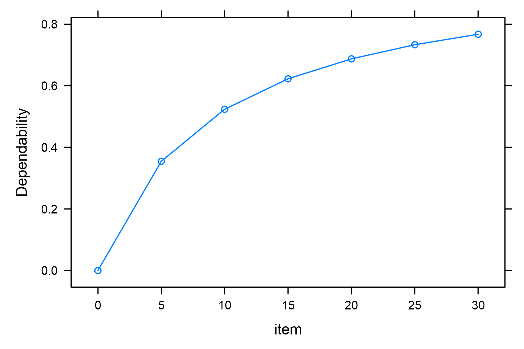
Finally, the dstudy_plot() function of the hemp package provides a visualization of generalizability and dependability coefficients based on a different number of items. We use the seq() function to specify the items as a sequence from 0 to 30 with a step of 5.
hemp::dstudy_plot(G_pxi, unit = "id", facets = list(item = seq(0, 30, 5)),
                  g_coef = TRUE)
hemp::dstudy_plot(G_pxi, unit = "id", facets = list(item = seq(0, 30, 5)),
                  g_coef = FALSE)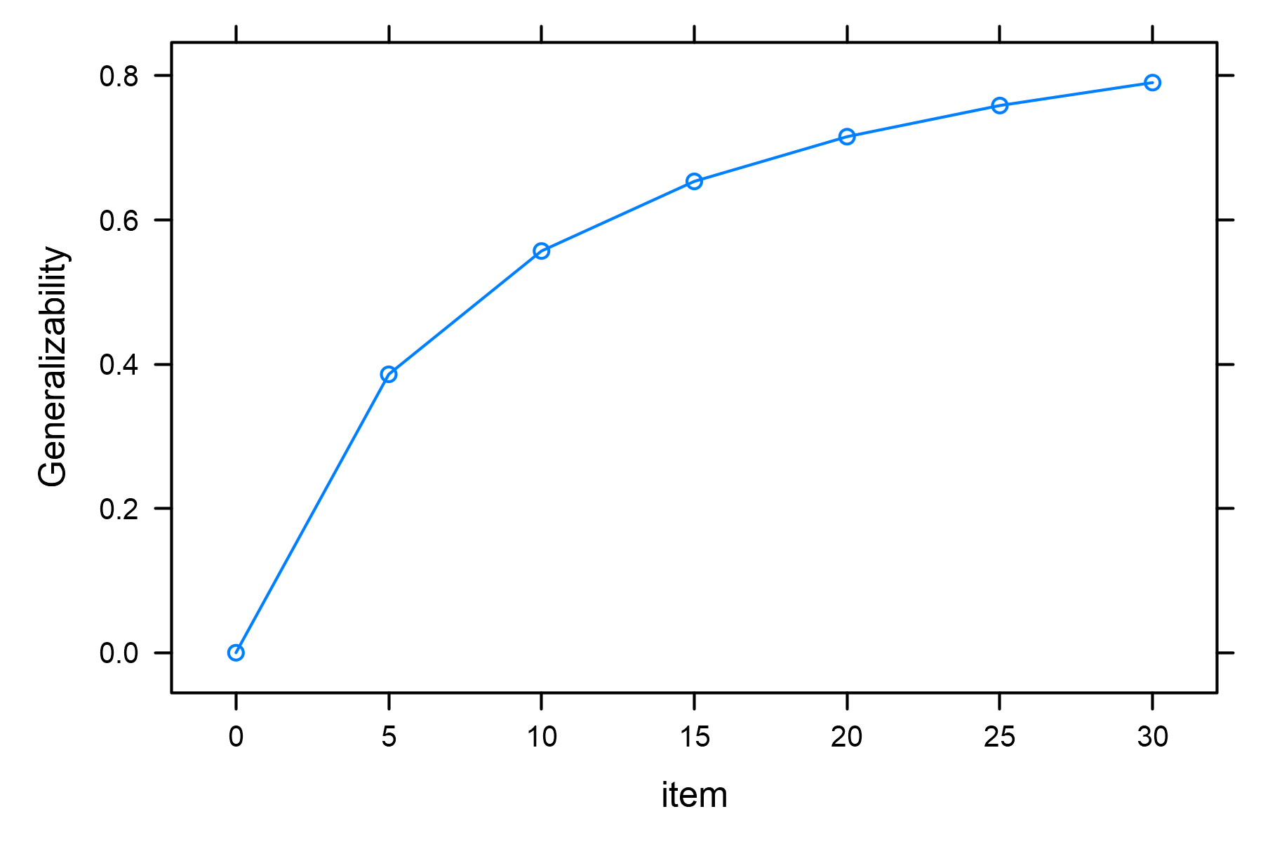
HCI dataset.
For example, to achieve the generalizability or dependability index of 0.40, roughly 5 items would be enough (Figure 4.5 (a)). On the other hand, 30 items would be needed to achieve a generalizability or dependability index of 0.80 (Figure 4.5 (b)).
4.4.2 A two-facet study
A two-facet study generalizes the one-facet study by one additional source of variance. This leads to a 3-way ANOVA model. As an example, we may consider students rated by multiple raters on multiple items, or grant applications rated by multiple raters on various criteria as in Erosheva et al. (2020). See the Supplementary R code and Exercise for examples of a two-facet G-study and D-study.
4.5 Other estimates of reliability
Cronbach’s alpha is based upon an assumption of essentially \(\tau\)-equivalent item measurements. In many practical situations and when measured trait is multidimensional, this assumption is not plausible, and a more relaxing assumption of congeneric item measurements needs to be considered. In such a case, the McDonald’s omega (Zinbarg et al., 2005) may be used as an alternative to Cronbach’s alpha.
Reliability under heterogeneity due to covariates. Reliability may be affected by contextual variables such as the gender or experience of the rater or ratee (Goldhaber et al., 2021; Martinková et al., 2018). Identification of such differences and identification of subgroups with low reliability may help in developing policies for increasing reliability by focusing on the most relevant subgroups. Martinková et al. (2023) developed a flexible Bayesian approach for assessing reliability in cases of heterogeneity due to covariates, and they provided a comparison with other possible approaches.
4.6 Reliability in interactive application
The ShinyItemAnalysis application offers implementation of the Spearman-Brown formula, providing predictions for reliability change with a higher or lower number of items or raters. It also provides several estimates of reliability including the split-half coefficients and Cronbach’s alpha (Figure 4.6).

ShinyItemAnalysis.
Spearman-Brown formula. Calculations made using the Spearman-Brown formula Equation 4.9 are provided within the Reliability section under the Spearman-Brown formula tab. The reliability and the number of items are pre-selected based on the currently uploaded dataset. The user can also specify other values of reliability and number of items. The default target test length is 10 items higher than the original length of the dataset; however the target length may also be specified by the user. The application then predicts the reliability of the prolonged/shortened instrument based upon these specifications.
The number of necessary items can be similarly calculated by providing the desired level of reliability of the new data.
Split-half coefficients. The ShinyItemAnalysis application provides a number of split-half approaches including first-second, even-odd, and others. Using the HCI dataset, the first-second method yielded a reliability of 0.697 (Figure 4.6). This value is rather low as can be noted from the histogram of all possible split-half coefficients. Contrarily, the even-odd approach gives a reliability of 0.742 (figure not shown), which is higher than the average reliability given by 10,000 split-halves.
Other possibilities include minimal split-half, maximal split-half, or average split-half. For the calculation of these, the software by default takes only 10,000 randomly selected split halves; however, the actual number of all possible splits is provided, and the number used can be changed by the user. The same number of splits is used for plotting the histograms.
Cronbach’s alpha. The ShinyItemAnalysis provides calculation of Cronbach’s alpha Equation 4.14 in the Reliability section under the tab Cronbach’s alpha. A confidence interval is calculated from the \(F\) distribution as outlined in Equation 4.18.
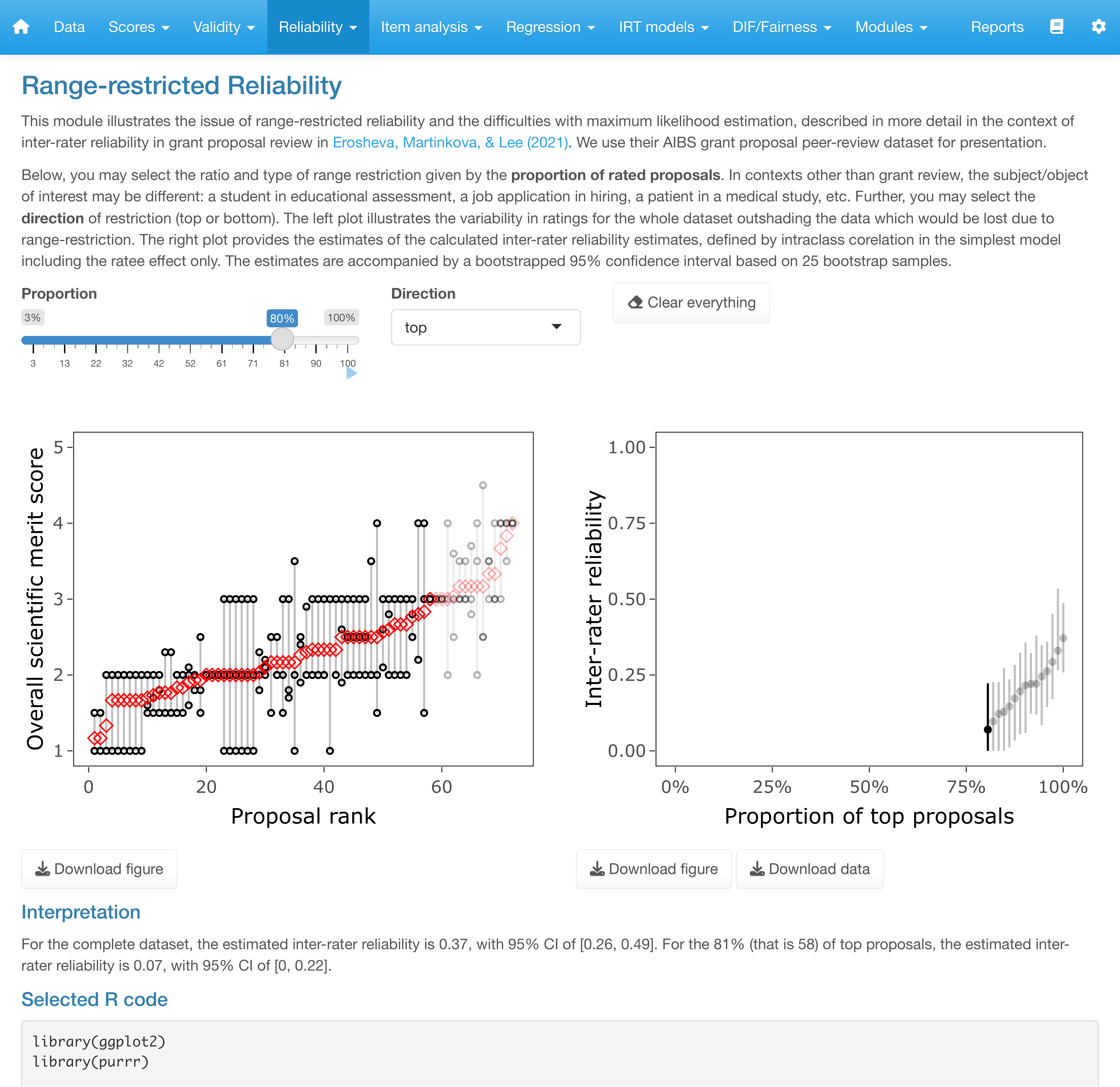
Reliability in restricted range. The issues with range restriction in reliability estimation are demonstrated in the Restricted-range reliability module of the SIAmodules package, accessible from the Reliability section (Figure 4.7). The module uses the AIBS grant peer review scoring data to provide a practical demonstration as presented in Erosheva et al. (2021). More information on the ShinyItemAnalysis modules is provided in Section A.6.1.
ShinyItemAnalysis module on IRR under range restriction.
4.7 Summary
In this chapter, we have discussed methods for enumerating the amount of error which is omnipresent in behavioral measurement, and how to collect proofs of measurement reliability. Reliability was defined using correlation coefficients, with Cronbach’s alpha under several frameworks, and estimates based on ANOVA, ML in mixed-effect regression models, and under Bayesian framework. Further extensions, including those to more sources of error, were presented. In the end, we have presented implementations in the interactive application.
See https://github.com/cddesja/hemp/ for instructions on how to install the package.↩︎