10 Selected Topics
10.1 Introduction
There are a number of other psychometric topics which may be of interest, but there is not enough space to analyze them more deeply in this book. In this chapter, we will touch upon some of these topics at least briefly. We start with two applications of IRT models presented in Chapter 7 and Chapter 8: In Section 10.2, we will present computerized adaptive testing which offers the possibility to select, at each step, an optimal item for the respondent, based upon their previous responses. In Section 10.3, we will discuss test equating and linking methods dealing with the case of multiple test forms. In Section 10.4, we will then focus on frameworks generalizing IRT models into more complex model classes. In Section 10.5, we will present more contemporary topics and computational psychometric methods which are receiving increasing attention with the rise of big data. We will finally discuss how demonstrations of further psychometric topics may be implemented interactively with modules for the ShinyItemAnalysis application.
10.2 Computerized adaptive testing
In the context of educational testing, student abilities may differ remarkably, and when taking a test, some students may become bored by questions which are too easy, while other students may become stressed by questions which are too difficult. In the context of psychological and health-related measurements, burdening the respondents with questions which are too far from their latent trait may cause fatigue. In all these scenarios, the selection of proper items may save time and lower test anxiety. Moreover, in high-stakes tests, test security is also of interest, and computerized tests have the potential to lower item leakage.
Before describing the algorithms behind adaptive tests, it is necessary to provide a wider overview of various test delivery models. The most traditional and popular test delivery model is a linear test, also called a fixed test, in which all test takers are presented with the same fixed set of items, one after another. Items can be presented in a different order or with reordered option choices to prevent certain types of cheating. More and more often in recent days, these tests are no longer paper-and-pencil tests, but rather CBT. This may bring some advantages: CBT will allow for scrambling item presentation at run-time, keeping track of item response time, quickly evaluating the test, and providing test feedback to the student shortly after completion.
The CAT, also called item-level CAT, which we will mostly focus on in this section, has the added advantage of computational psychometrics: After administration of each item, an estimate of respondent ability is updated. Subsequently, using information about the properties of those items currently available in an item bank provides the optimal item for selection at the moment. As a result, the CAT can often estimate ability with the same precision using half the items required by a linear test.
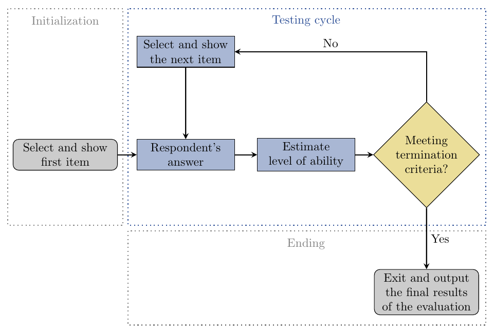
To provide additional details, the CAT is composed of three phases: a) Initialization, b) Testing cycle, and c) Ending (Figure 10.1). In the initialization phase, an estimate of the respondent’s ability is obtained. This is based upon either an answer to an initial item(s), a pretest, or in some other way. The testing cycle then moves to selecting an optimal item and gathering a response, updating the respondent’s ability estimate, and checking the precision of the estimate or some other termination criteria. These steps are repeated until the termination criterion is met. Once this is completed, the testing cycle is concluded, and, in the ending phase, an algorithm provides the final ability estimate, or the final classification of the respondent into an ability category if that is of interest.
Other test delivery models are possible; see for example Drasgow (2015). Notably, the MST is a compromise between a linear test and the CAT. The MST updates an estimate of the respondent’s ability after a block of items which will decide the next set of items presented to the respondent in the following stage of the test. This approach combines the advantages of item-level CAT and those of fixed tests: On one hand, test anxiety is lower and the precision of an ability estimate is higher given the number of items presented to the respondent. On the other hand, the respondent can go back and correct their items within the block of items presented to them (which is not possible in an item-level CAT). It also provides more explicit control over test form quality, content validity, and item exposure. For further details on CAT and MST, the reader is referred to Magis et al. (2017).
10.2.1 Item bank
To assure proper functioning of the adaptive test, a high number of items is needed to be available in an item bank. The item bank should be based upon test specifications and should include a sufficient number of items for each content category. All items in the item bank should be reviewed by content experts, and new items should preferably be pretested and analyzed using the psychometric models and methods described in earlier chapters. Only well-functioning items should then be selected for further use. The item bank needs to be regularly re-evaluated for size, specifications, and content balance, and new items should be added regularly depending upon the intensity of test administration.
Item calibration is an important element when building the item bank: To run CAT, item parameters are needed for each item. These can be gathered from previous use of the item with a population of respondents possessing the same characteristics as the population of interest. We focus here on the CAT based upon IRT models. For running these, parameter estimates using an appropriate IRT model are necessary. For details on item parameter estimation under the IRT framework, see Section 7.3.
10.2.2 Ability estimation
Ability estimation under the IRT framework was discussed in detail during Section 7.3. A ML estimate of ability \(\theta\) is computed after each step of the CAT algorithm. In the case of binary items, the ML estimate \(\hat{\theta}_{\text{ML}, k}\) maximizes the likelihood function \[ L(\boldsymbol{\xi}, \theta) = \Pr(\boldsymbol{Y} = \boldsymbol{y}|\theta, \boldsymbol{\xi}) = \prod_{i \in A_k} \pi_{i}^{y_{i}} (1 - \pi_{i})^{1 - y_{i}}, \] where \(\boldsymbol{\xi}\) is a matrix of the known item parameters and \(\boldsymbol{y}\) is a vector of binary responses from one respondent to a set of items \(A_k\) administered before step \(k\).
Note that in the early stages of a CAT, ability estimation is performed based upon only a limited number of items. This implies that the ML estimate may easily return infinity values, which is the case whenever there is no variability in item responses, i.e., all item responses are either correct or incorrect. For this reason, other approaches need to be considered, such as weighted ML or Bayesian estimates which eliminate infinite estimates by using a prior distribution, at least until some variability in item responses is present; see Section 7.3.4.1 for more details.
10.2.3 Item selection algorithms
The effectiveness of a CAT may depend upon the item selection algorithm. The linear test may be formulated in terms of a CAT with a naive sequential (non-adaptive) criterion. Random selection of items may be similarly considered. The so-called Urry’s criterion (Urry, 1977) suggests using an item from the pool of available items which is closest in difficulty to the respondent’s current ability estimate. Using a 1PL IRT model, selecting an item using the Urry’s criterion is equivalent to selecting an item with the highest information for the respondent’s currently estimated ability level.
A number of selection criteria are based upon Fisher information. In his seminal work, Lord (1977) considered the MI criterion. This criterion can be applied to any IRT model. By using this criterion, for a given ability estimate, an item with the highest information at the respondent’s currently estimated ability level is selected. As described earlier in Section 7.3.6, Fisher information Equation 7.17 contains no reference to the observed response patterns, and it provides the expected information of currently available items given the ability level \(\theta\). However, the true value of \(\theta\) is not available, and its current estimate \(\hat{\theta}\) is used, which as mentioned above, can be highly imprecise, especially for the initial steps. This issue is overcome by using alternative approaches: The MLWI criterion maximizes the information weighted by the likelihood function of the items already administered. Alternatively, the MPWC uses posterior distribution as the weighting function.
Instead of maximizing the information function over the current available items, the MEI and the MEPV criteria use an expected optimal function based upon the possible responses to the next item administered. In both cases, the probabilities of answering the next item correctly or incorrectly are calculated, and the response pattern is updated conditionally upon these two possible responses. In the case of the MEI criterion, the expected information function is maximized for the selected items. For the MEPV, the expected posterior variance for the ability level of the selected item is minimized.
Exposure rate control. To avoid some items from being exposed too many times, exposure rate control algorithms may be implemented in item selection. In one algorithm (so-called randomesque), the item is randomly selected from a set of optimal \(k\) items. Another option is to randomly select from a set of items which are descending in number (so-called 5–4–3–2–1 method). Finally, the so-called Sympson-Hetter method works as follows: An exposure ratio \(r_i^{\text{max}} \in (0, 1]\) is predefined for each item. If an item is selected as an optimal item for respondent \(p\), a random value \(r_{p, i}\) is simulated from a uniform distribution on \((0, 1).\) In the case of \(r_{p, i} \leq r_i^{\text{max}}\), the selected item is assigned; otherwise it is discarded for respondent \(p\) and not assigned to this respondent in any future steps.
Content balancing. Item selection algorithms may also need to incorporate content balancing, in order to keep the topics in the test balance and to ensure content validity. Assuming that an item bank is divided into content categories and that a predefined optimal ratio of items is specified, a simple algorithm may be considered for content balancing. At each step of the CAT:
- The current ratio of each content category is calculated,
- The content category with the highest difference between current and requested ratio is identified,
- The next optimal item is selected from this category.
10.2.4 Stopping rules
Different stopping rules may be implemented. The easiest stopping criterion considers a test length: The test is terminated if a preset number of items was answered by the respondent. Alternatively, a test may be terminated when the ability estimate precision criterion, in terms of a minimal standard error in the ability estimate, is met. Finally, in tests where the main objective is to categorize the respondents (such as criterion-reference tests or certification tests), the test is stopped when the ability confidence interval is completely above or completely below the threshold level. The stopping rules may be combined; for example, the length criterion and the estimate precision criterion may be jointly applied.
10.2.5 CAT implementation in interactive application
In R, a CAT can be implemented as an interactive Shiny application with the mirtCAT() function of the mirtCAT package. As the first input, the function takes a data.frame object which can include wording of the items, wording of the options in the case of multiple-choice or Likert-scale items, correct answers, types of items; it may also include specification of time available for each item and other options. For our demonstration of CAT implementation, we use the items automatically generated to test elementary arithmetic, specifically the multiplication tables from 1 to 10 (see Supplementary R code for item generation). Item wording together with further specification is organized into a data frame:
df <- data.frame(Question = Question, Answer = Answer, Type = Type,
                 stringsAsFactors = FALSE)
head(df, n = 2)
##     Question Answer Type
##  1 1 * 1 = ?      1 text
##  2 1 * 2 = ?      2 text
As the second input, the mirtCAT() function takes an IRT model. In our demonstration example, we defined item difficulty parameters so that multiplication by 1 is considered the easiest, followed by multiplication by 10, etc. (see Supplementary R code). These difficulty parameters are used to generate a mirt object using the generate.mirt_object() function of the mirtCAT package. We use a 1PL IRT model by setting the discrimination parameters at a value of 1, i.e., a1 = 1. The difficulty is applied with an opposite sign since the mirt and mirtCAT packages use intercept-slope parametrization:
library(mirtCAT)
pars <- data.frame(a1 = 1, d = -Diff)
model <- generate.mirt_object(pars, itemtype = "2PL")
The item parameters, ICC, and IIC for each item of the generated model can be printed and displayed with the coef() and plot() methods as was shown in Chapter 7 (see Supplementary R code).
The mirtCAT() function further allows for some additional settings. In our demonstration, we set the argument method = "MAP" to specify that ability is to be estimated at each step with the MAP method (see Section 7.3.4.1). The item selection criteria is set to the MI by the argument criteria = "MI". An argument design is used to set the stopping rule at a combination of the maximum number of items allowed and the minimum standard error of \(0.6\) of the respondent’s ability. The mirtCAT() function directly opens up the defined interactive CAT (Figure 10.2). In the code below, the responses are saved into the result object.
results <- mirtCAT(df, mo = model, method = "MAP", criteria = "MI",
                   design = list(max_items = 10, min_SEM = 0.6))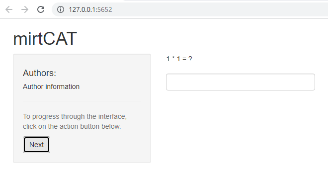
In our demonstration, we have answered the first, sixth, and eighth (last) items correctly, and we have otherwise entered a wrong answer (blank space). After finishing the test and closing the browser, the results are saved. A print of the output shows the number of items answered, an estimate of ability (in this case we have only a one-dimensional ability; thus only one Theta value is provided), and its standard error.
print(results)
##  n.items.answered  Theta_1  SE.Theta_1
##                 8  -0.8352     0.5886
The summary() method provides a more detailed summary of the results including the raw item responses, scored responses, item numbers presented to the respondent, and a step-by-step history of the ability estimate with its standard error.
summary(results)
##  $final_estimates
##  Theta_1
##  Estimates -0.8352
##  SEs        0.5886
##
##  $raw_responses
##  [1] "1"  " "  " "  " "  " "  "20" " "  "30"
##
##  $scored_responses
##  [1] 1 0 0 0 0 1 0 1
##
##  $items_answered
##  [1]   1 54 24 12 92 20 93 30
##
##  $thetas_history
##  Theta_1
##  [1,]  0.0000
## ...
##  [8,] -1.0098
##  [9,] -0.8352
##
##  $thetas_SE_history
##  Theta_1
##  [1,] 1.0000
##  ..
##  [8,] 0.6185
##  [9,] 0.5886
##
##  $terminated_sucessfully
##  [1] TRUE
As expected, the standard errors of the ability estimates get smaller with each additional item answered. After answering the eighth item, the standard error finally fell below the stopping criterion of \(0.60\), and the CAT successfully terminated.
Progress of the ability estimation and standard errors of the estimates can be displayed with the plot() method (Figure 10.3). Argument SE = 1.96 can be used to display 95% confidence intervals instead of the standard errors (not displayed).
plot(results)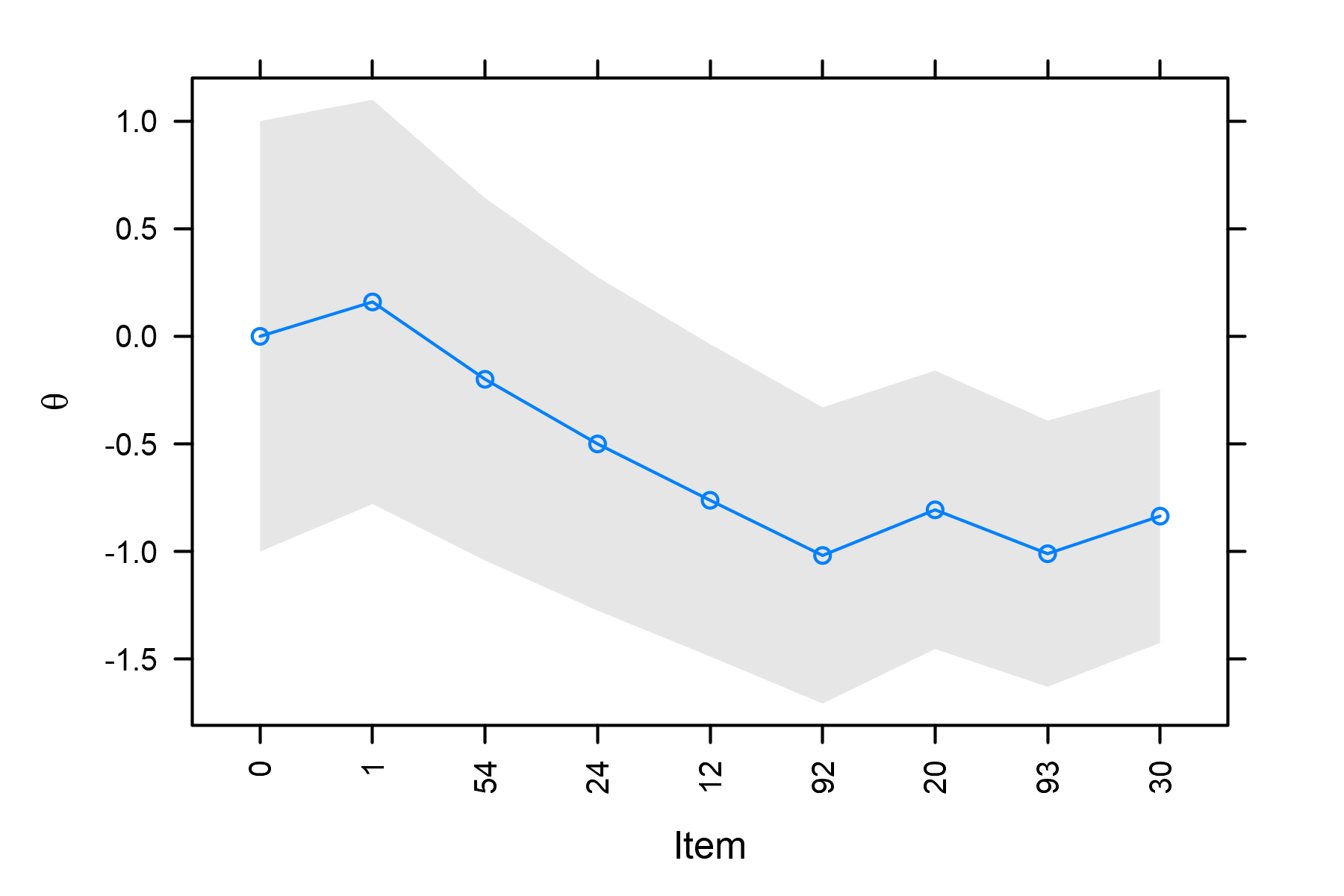
A number of further options for the implementation of CAT with the mirtCAT() function are available, including different settings of the graphical display, pretest definition, item time constraints, content balancing, or exposure control (see Supplementary R code).
Other software packages which allow for CAT implementation are catR and catIRT. For example, CAT can be implemented by combining the catR package with the open-source Concerto platform1.
10.2.6 Post-hoc analysis
We have so far presented how CAT can be implemented when a pre-calibrated item bank is available. We discussed different settings, such as termination criterion, item selection algorithms, and others. To research how these settings compare to each other, and how the CAT compares with a linear test on a certain assessment type, it is useful to perform a so-called post-hoc analysis or post-hoc simulation.
The post-hoc analysis is a simulation of an adaptive test created after the respondents answered all available items in a linear test. The item parameters can be predefined or estimated based upon the data collected from a linear test. A simulation follows the selected settings of an adaptive test – an initial estimate of ability, item selection, predefined stopping rule, or other selection. In each step, according to defined CAT settings, an algorithm selects the optimal item, checks what the respondent’s answer was for this item in a linear test, uses this answer to obtain an updated ability estimate and its standard error, and checks if the stopping criterion is met. If these requirements are not reached, a new item is selected and the algorithm continues. Once the stopping rule is met, a final estimate of ability is returned. If the stopping rule is not met after using all the available items, the simulation ends after reaching the maximal number of items.
To present a practical example of a post-hoc analysis, we follow Štěpánek & Martinková (2020) using a 100-item dataset from a medical school admission test dataMedical.
data("dataMedical", package = "ShinyItemAnalysis")
data <- dataMedical[, 1:100]
We use the mirt() function of the mirt package to estimate item parameters, under the 2PL IRT model Equation 7.3, as was more completely described in Section 7.4.1. The ICCs and IICs are plotted with the plot() method.
library(mirt)
fit2pl <- mirt(data, model = 1, itemtype = "2PL", SE = TRUE)
coef(fit2pl, IRTpars = TRUE, simplify = TRUE)$items
##            a       b g u
## X2001 0.2751  2.8194 0 1
## X2002 0.6036  4.1328 0 1
## X2003 1.0267  0.5342 0 1
## ...
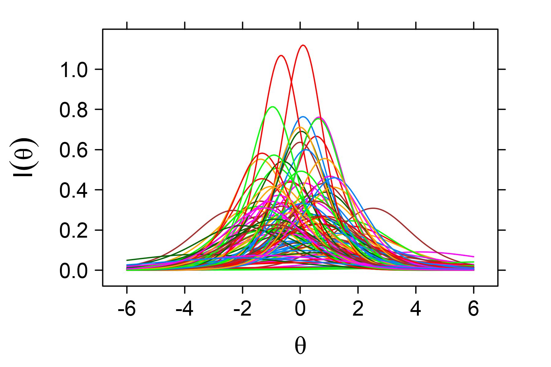
plot(fit2pl, type = "trace", facet_items = FALSE)
plot(fit2pl, type = "infotrace", facet_items = FALSE)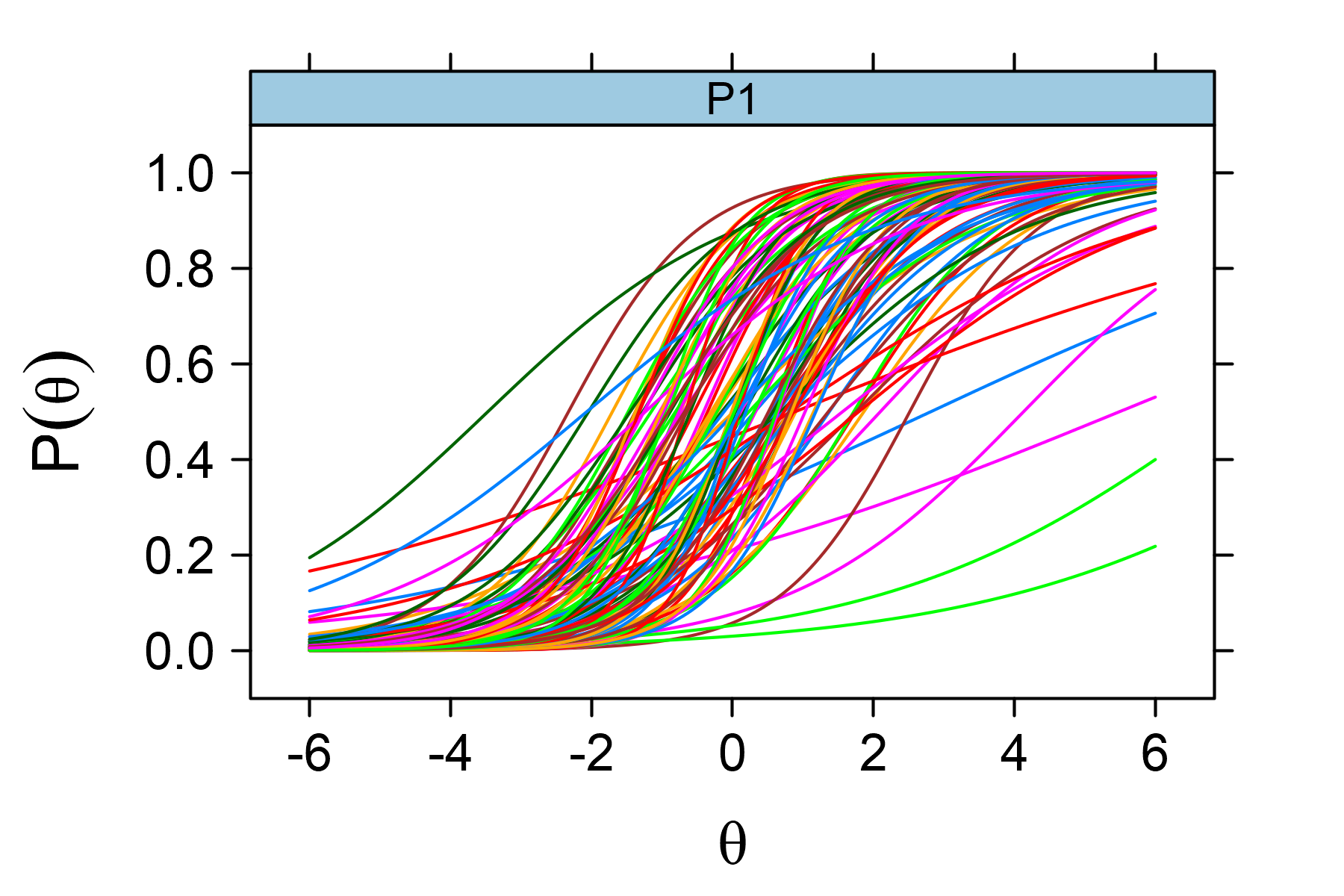
dataMedical dataset.
The resulting ICCs and IICs suggest that the items are functioning well, and for levels of ability on interval \((-3, 3)\), there are a number of informative items (Figure 10.4).
Post-hoc CAT analysis with the mirtCAT package. We present here two illustrations of the post-hoc simulation with the mirtCAT() function of the mirtCAT package. In the first illustration, we use the 2PL IRT model fitted above by specifying the argument mo = fit2pl. We select data from the first respondent with argument local_pattern. The first item selected will be the one with maximum observed information for an average ability (argument start_item = "MI"). At each step, the ability estimate will be obtained using the MAP method (argument method = "MAP"), and the next item will be selected with the MI criteria method (criteria = "MI"). The stopping criterion is defined as a minimal standard error of 0.30 by specifying min_SEM = 0.30 in the design argument. This level was chosen based upon standard errors of ability estimates from a complete set of items (see Figure 4 in Štěpánek & Martinková, 2020), and it also corresponds to reliability of \(1 - 0.30^2 = 0.91\), see Equation 4.6.
posthocSim1 <- mirtCAT(mo = fit2pl, local_pattern = data[1, ],
                       start_item = "MI", method = "MAP",
                       criteria = "MI", design = list(min_SEM = 0.30))
We then use the print() and summary() methods to display results of the post-hoc analysis.
print(posthocSim1)
## n.items.answered Theta_1 SE.Theta_1
##               19  0.3609     0.2976
summary(posthocSim1)
## $final_estimates
## Theta_1
## Estimates  0.3609
## SEs        0.2976
## $raw_responses
## [1] "2" "1" "1" "2" "2" "2" "1" "1" "1" "2" "1" "1" "2" "2" "2" "2"
##     "2" "1" "2"
## $scored_responses
## [1] 1 0 0 1 1 1 0 0 0 1 0 0 1 1 1 1 1 0 1
## $items_answered
## [1] 81 72 57 82 73 76 18 78 56 74 90 30 80 53 89 37 70 79 69
## $thetas_history
## Theta_1
##  [1,]  0.0000
##  [2,]  0.5691
## ...
## [20,]  0.3609
## $thetas_SE_history
## Theta_1
##  [1,]  1.0000
##  [2,]  0.7292
## ...
## [19,]  0.3012
## [20,]  0.2976
For the first respondent, the post-hoc analysis suggests that if they were given the test adaptively, the first item presented would be 81, which we know they answered correctly. This would shift the estimate of their ability from 0 to 0.57 and lower the standard error for their ability estimate from 1 to 0.73. The next item, optimal for their ability level, that would be offered to this respondent is item 72. They answered this item incorrectly. Altogether, 19 items would be presented to this respondent before the standard error of their final ability estimate was below the threshold of 0.3. This is a considerably lower number of items than the complete set of 100 items. In this case the final ability estimate is 0.36 (SE = 0.29).
The plot() method for the output of the mirtCAT() function shows estimates of ability for respondent 1 when the test was given adaptively together with standard errors. The x-axis provides the ID numbers of items which would be presented to the respondent (Figure 10.5 (a)).
plot(posthocSim1)As a second example, we consider the same setting but with a different termination criterion. Instead of using the ability estimate precision rule, we will now consider a classification task for a cut-score \(-0.1\) with a 90% confidence interval as the stopping criterion by specifying the classify = -0.1 and classify_CI = 0.90 in the design argument. We can again use the print() method to display the results of the post-hoc analysis, and the summary() method to display further details (see Supplementary R code).
posthocSim2 <- mirtCAT(mo = fit2pl, local_pattern = data[1, ],
                       start_item = "MI", method = "MAP", criteria = "MI",
                       design = list(classify = -0.1, classify_CI = 0.90))
print(posthocSim2)
## n.items.answered Theta_1 SE.Theta_1
##               20  0.4210     0.2947
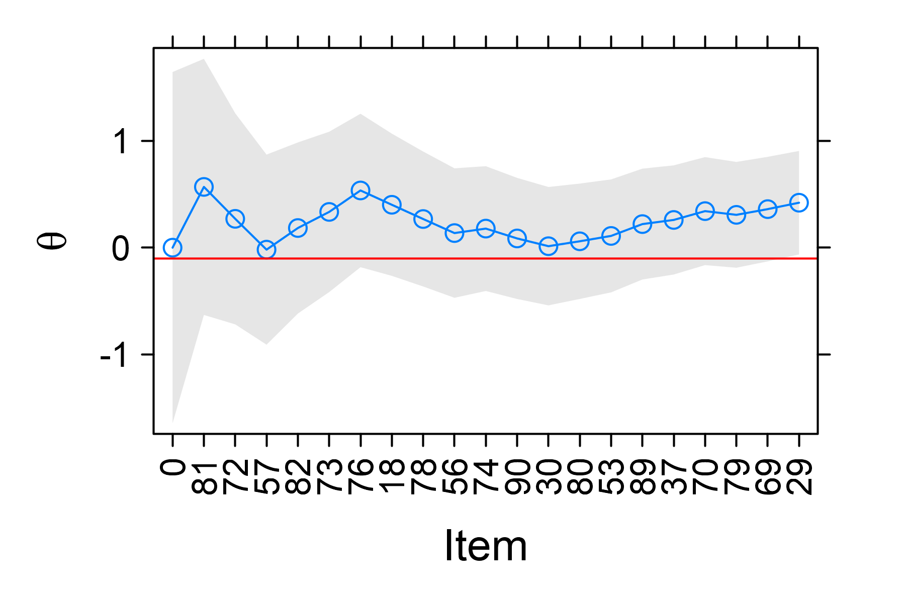
With this termination criterion, 20 items are presented to the first respondent before the final ability estimate and its 90% confidence interval was above the cutoff value of \(-0.1\). In this case the final estimate is 0.42 (SE = 0.29). To verify that the algorithm correctly ended after the termination criterion was met, we calculated the 90% confidence interval using a quantile of a normal distribution calculated with the qnorm() function.
posthocSim2$thetas - qnorm(0.95) * posthocSim2$SE_thetas
## [1,] -0.0637
posthocSim2$thetas + qnorm(0.95) * posthocSim2$SE_thetas
## [1,] 0.9058
As can be seen, the 90% confidence interval does not reach the threshold of \(-0.1\), while this was not the case at the previous step (Exercise 10.3).
In the plot() method of the mirtCAT() function, the 90% confidence intervals for the ability estimates can be displayed using the same quantile as used in our calculation above (Figure 10.5 (b)):
plot(posthocSim1, SE = qnorm(0.95))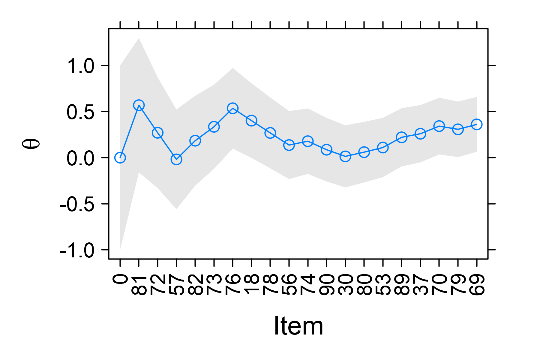
dataMedical dataset with various stopping criteria.
As expected, given the same ability estimation method and the same item selection algorithms implemented, in both post-hoc simulations, the items were presented in the same order and the same ability estimates were obtained in each step. Differences in the stopping criteria caused a different number of presented items: The second simulation required one extra item before the classification criterion was met (Figure 10.5).
The catR package is another option for performing a post-hoc analysis with its simulateRespondents() function (see Supplementary R code).
10.2.7 CAT simulation study with MCMC
The data are not necessarily needed for an evaluation on the feasibility of an adaptive test with items of given characteristics. The MCMC simulation study offers the possibility to explore the feasibility of an adaptive test based solely upon item parameters, which can be obtained from an earlier study. In the MCMC simulation study, the abilities of respondents are generated using an underlying distribution, such as a standard normal distribution.
CAT simulation study with MCMC in R. In the code below, we generated latent normally distributed abilities of 100 respondents by using the rnorm() function. We used the set.seed() function with an arbitrary seed 123 for replicability.
set.seed(123)
thetas <- rnorm(100)
Responses of these “hypothetical” respondents are then generated using a selected IRT model using the simdata() function of the mirtCAT package. The Z-scores are calculated based upon these simulated responses using the scale() and the rowSums() functions, as we had done in other chapters of the book. The correlation between true abilities and the Z-scores is estimated using the base cor() function.
responses <- simdata(model = fit2pl, Theta = as.matrix(thetas))
Zscores <- scale(rowSums(responses))
cor(thetas, Zscores)
## [1,] 0.9682
As expected, the correlation is very high, close to one (also see Supplementary R code for graphical display).
We can now use the simulated response data to simulate a CAT as we did before in Section 10.2.6. To add complexity, we will run the simulation for all “hypothetical” respondents, not just the first one. This is done using the lapply() function: For each simulated respondent p, from 1 to the sample size of 100, the mirtCAT() function is run with the same setting as in Section 10.2.6, and the results are saved into the MCMCsim list; therefore, the pth element of the list, MCMCsim[[p]], includes results of the pth respondent. We used the same CAT settings as we did in Section 10.2.6.
MCMCsim <- lapply(1:100, function(p)
    mirtCAT(mo = fit2pl, local_pattern = responses[p, ], start_item = "MI",
            method = "MAP", criteria = "MI", design = list(min_SEM = 0.30)))
The CAT results for a single respondent can be displayed as they were in Section 10.2.6.
thetas[1]
## [1] -0.5605
print(MCMCsim[[1]])
## n.items.answered Theta_1 SE.Theta_1
##               23 -0.8921     0.2963
For the first hypothetical respondent, who was simulated to have a true ability of \(-0.56\), 23 items would be used in the CAT specified above, and the resulting ability estimate would be \(-0.89\) (SE = 0.30).
To study the CAT suitability in more detail, we can now analyze CAT results from all hypothetical respondents. We will use the sapply() function to extract estimated abilities, their standard errors, and the number of items presented to each respondent. We will then explore and display them against the true abilities (Figure 10.6; also see Supplementary R code).
CAT_thetas <- sapply(MCMCsim, function(x) x$thetas)
cor(thetas, CAT_thetas)
## [1] 0.9523
cor(Zscores, CAT_thetas)
## [1] 0.9557

CAT_SE <- sapply(MCMCsim, function(x) x$SE_thetas)
summary(CAT_SE)
##   Min. 1st Qu.  Median    Mean 3rd Qu.    Max.
## 0.2928  0.2968  0.2984  0.2983  0.2990  0.3560
sd(CAT_SE)
## 0.0061

CAT_items <- sapply(MCMCsim, function(x) length(x$items_answered))
summary(CAT_items)
##  Min.    1st Qu.  Median     Mean   3rd Qu.    Max.
##  18.00    19.00    20.00    24.74    25.00   100.00
sd(CAT_items)
## [1] 13.0420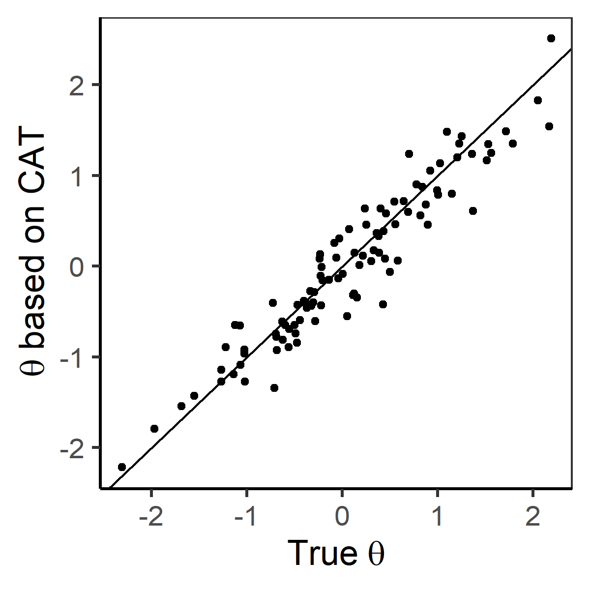
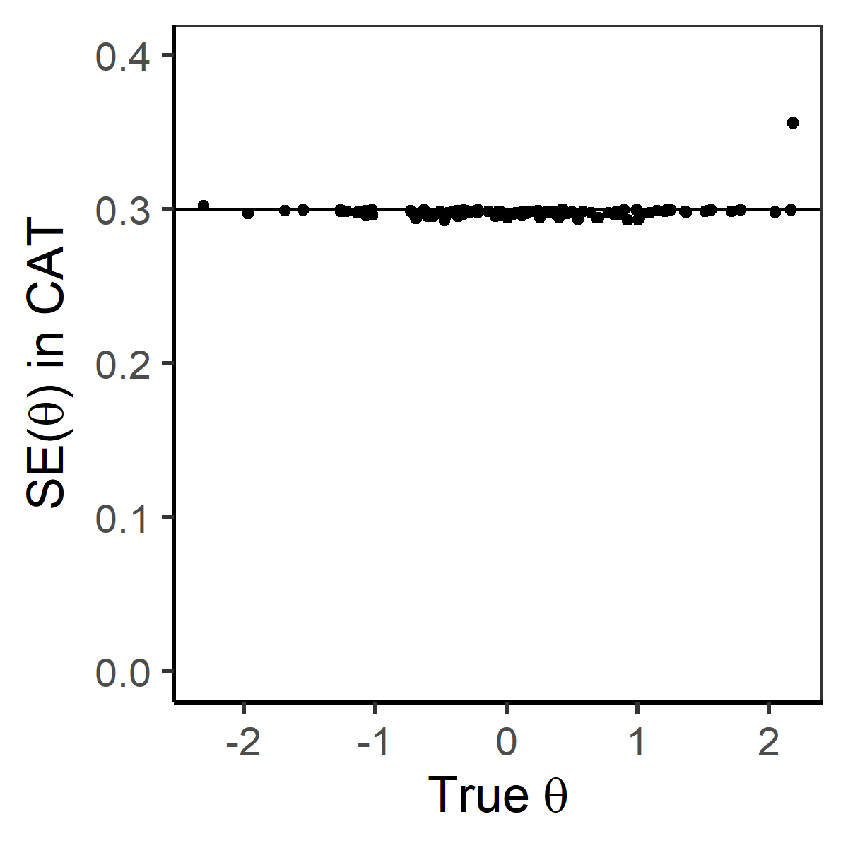
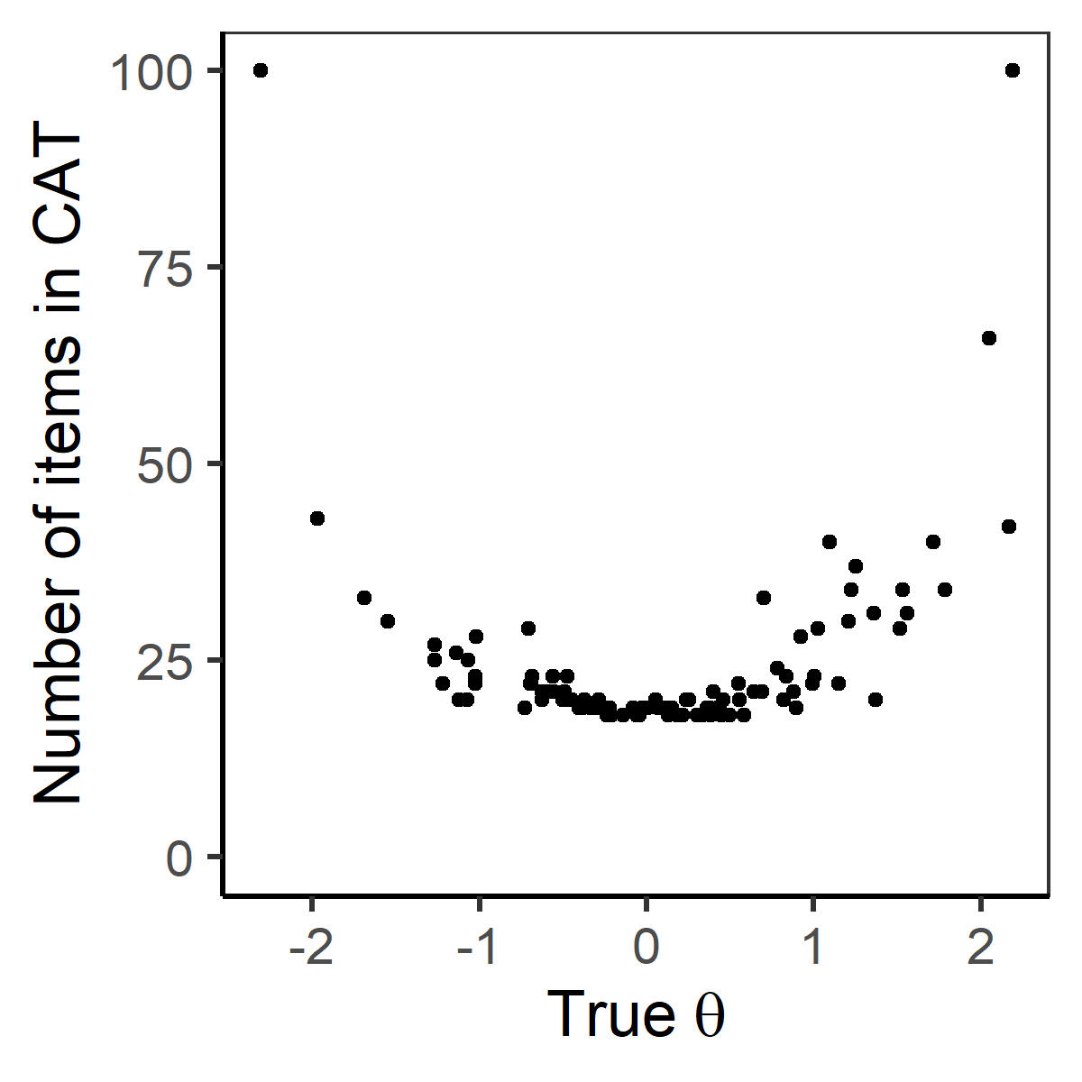
Abilities estimated from the CAT correlate very strongly with the underlying true abilities which were used to generate the item responses: The correlation of 0.95 is close to 1 and is only slightly lower than the correlation of 0.96 between the true scores and Z-scores calculated from all 100 responses (see Figure 10.6 (a)). Because of the CAT design (the stopping criterion), standard error was close to 0.30 for most simulated respondents, and it was above this threshold in only the two extreme cases where 100 items were not enough (Figure 10.6 (b), horizontal line representing the termination criterion threshold of 0.30). The number of items used was, in most instances, much lower than 100 (mean = 24.74, SD = 13.04). All 100 items were only needed for (simulated) respondents with abilities very far from 0, for which the item bank most likely did not contain enough suitable items. For abilities close to 0, less than 30 items were sufficient (Figure 10.6 (c)).
The catR package is another option for performing a MCMC simulation using its randomCAT() function in combination with the simulateRespondents() function. The strength of the catR package is a plotting method which offers a number of informative graphical displays (see Supplementary R code).
The presented simulation study described only the single CAT design. Further possibilities for the evaluation of a CAT simulation include comparison of different settings (i.e., different stopping criteria, different item selection criteria, etc., see Exercise 10.4). This would add additional layers to plots presented in Figure 10.6 and may help uncover optimal settings for specific testing situations (Tělupil, 2018). Other relationships could also be displayed using different settings. These settings may include the exposure rate of individual items or the time needed to run the CAT.
10.3 Test equating and linking
When an assessment is done using different test forms, potentially of slightly different difficulty, and/or on different groups of respondents with possibly different ability levels, the estimates of person abilities and item parameters will most likely be on different metrics. The process of adjusting the person ability estimates in order to place them on the same metrics is known as equating.
Traditional equating methods use mean, linear, or equipercentile equating transformations under different data collection designs, including single group, equivalent groups, counterbalanced group design, and others. These approaches transform the ability estimates of one test form to those of another test form to align the means, means and variances (for linear equating), or all percentiles (for equipercentile equating), depending upon the method selected. Total scores, which are typically of a discrete nature, are usually subject to continuization prior to applying the appropriate equating method. For a general overview of equating methods, the reader is referred to Kolen & Brennan (2014), while more specific topics and details can be found in Davier (2010).
Kernel equating (Davier et al., 2004) offers a collection of methods in which kernel smoothing techniques (Silverman, 1981) are used to obtain continuous approximations of total score distributions. Non-equivalent group designs can be equated with anchor tests (subsets of items assigned to multiple groups) using traditional equating approaches or IRT-based equating methods. If no anchor test is available, respondent characteristics (covariates) may be used as a proxy (Wiberg & Bränberg, 2015).
The R packages offering equating methods include SNSequate (González, 2014), equate (Albano, 2016) for traditional equating methods, kequate (Andersson et al., 2013) focusing on kernel equating methods, and equateIRT (Battauz, 2015) focusing on IRT-based methods. For more details about applying test equating methods with R, the reader is referred to González & Wiberg (2017).
10.4 Generalizing latent variable models
The FA models presented in Section 9.6.3, the IRT models introduced in Chapter 7 and Chapter 8, as well as group-specific IRT models discussed in Section 9.5 belong to a wider class of latent variable models and may be encompassed in a more unified approach to be further generalized. The unified approach covers different response types (items) in the measurement model. Besides continuous, binary, or ordinal response types discussed in previous chapters, other possibilities include time duration such as item response time, comparative measurements such as rankings or pairwise comparisons, counts, or mixed responses. Similarly, the latent variables may not only be continuous, as we assumed in previous chapters, but also categorical, as is assumed in latent class models or in cognitive diagnosis models.
The SEM (Bollen, 1989; Kaplan, 2009) use measurement models as building blocks while focusing on relationships between variables, some of which may be latent. Further generalizations include the multilevel latent variable models in which the latent variables may be hierarchical. Longitudinal models are helpful in situations when the same respondents are measured repeatedly at a number of time occasions, and predictions of changes in responses and in latent variables over time is of interest. The typical feature of these models is that they account for both the dependence between answers of the same respondent, and time-varying influences which cause greater dependence between those responses occurring closer in time. Various longitudinal models may be defined, such as a latent growth model or a two-tier model (Cai, 2010), depending upon the choice of dependence structure.
For more details on further generalizations and a more unified approach to latent variable modeling, the reader is referred to Bartholomew et al. (2011) and Skrondal & Rabe-Hesketh (2004).
10.5 Big data and computational psychometrics
With the rise of computerized testing, technology-enhanced learning and assessment systems and electronic devices, the complexity of the data collected in psychological, educational, health, and other measurement increases tremendously. While most of the psychometric methods were developed for relatively simple data forms such as those collected with multi-item questionnaires, the recent era offers more detailed data, possibilities to integrate assessment with learning, analyze the results over time and place, and connect assessment with multiple sources of data (Davier et al., 2021). For example, when examining the ability to solve problems in technology-rich environments, besides the correctness of the item response, the so-called process data may be of interest, providing a detailed record of a respondent’s interaction with the system, including all respondent actions together with time stamps. Eye-tracking data may provide more details on distractors which most attracted the respondent. Functional magnetic resonance imaging (fMRI) or electroencephalogram (EEG) data may be used to analyze brain activity during a task.
The increased complexity of available data goes hand in hand with the increased complexity of the algorithms implemented. The computational psychometrics thus blend data science techniques, computer science, and psychometric approaches to analyze such complex measurement data. The algorithms involved include machine learning algorithms, text mining, and natural language algorithms allowing for the extraction of information from huge text files or to automatically create new items (Davier et al., 2021).
The use of personal electronic devices and social networks implies a huge amount of digital footprints created by the users (Rust et al., 2021) which, when combined with other personal data, provide detailed respondent information. Such complex and detailed data combined with artificial intelligence and machine learning algorithms offer more precise estimates of abilities, allowing for the prediction of human behavior and affording the opportunity to study it in more detail, while still supporting the development of traditional measures. Besides the computational aspects and challenges connected with analysis of the data, which we focused on in this book, and further possibilities which we mentioned in this final chapter, the rise of big data also brings ethical challenges connected with privacy, control, and use of the data we leave behind.
10.6 Interactive psychometric modules
The interactive application of the ShinyItemAnalysis package covers the main psychometric topics presented in each chapter of this book. As was presented in previous chapters, it offers a set of toy datasets, but it also allows the user to upload their own data and run covered psychometric analyses on these uploaded data. The application currently allows for the upload of item data with binary, ordinal, and nominal items with a key used for scoring, while for some analyses the scored or ordinal data are treated as continuous. It is also possible to upload vector data of a grouping variable, external observed ability, or a criterion variable.
As was explained in this last chapter, further psychometric topics often involve more complex data structures, including multiple time points, response-time data, multiple test versions, etc. Before further topics are directly implemented and the required data structures are offered within the main interactive application, it is possible to embed interactive presentations of these advanced topics as ShinyItemAnalysis modules, an example of which we present here.
A ShinyItemAnalysis module shares the same design as the main interactive application. It can use either a single toy dataset, multiple toy datasets, or it can even offer its own data upload. As an example, we present here a ShinyItemAnalysis module of the SIAmodules package for the topic of a CAT using post-hoc simulation presented in Section 10.2.6. While the module is developed separately and stored in an external package, the ShinyItemAnalysis application can offer it in the Modules tab of the main application (Figure 10.7), or even in other tabs, as specified in the package.
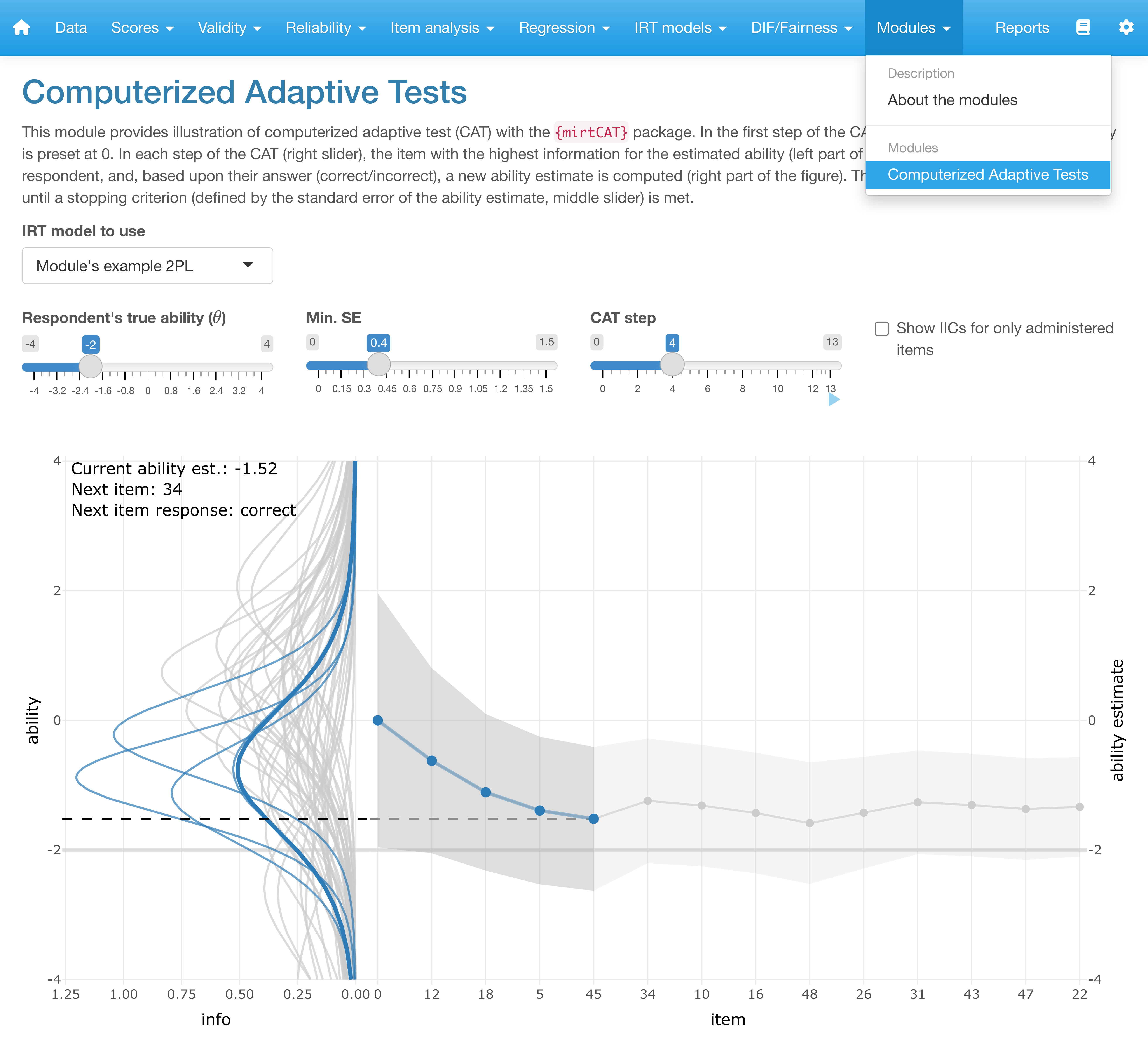
ShinyItemAnalysis module on CAT.
As with the case in the main interactive application, this module provides a general introduction to the topic (here the topic of adaptive testing) which may include a reference, an interactive demonstration of the topic with an interpretation, and possibly also a selected R code for the analysis (see also the module on reliability under the range restriction in Figure 4.7). In the future, other psychometric topics may be added into the ShinyItemAnalysis interactive application.
10.7 Summary
In this chapter, we have discussed applications of IRT models and other existing and emerging topics in psychometrics. We have first focused on a CAT, an approach in which test items are tailored to respondent’s ability based upon their previous responses. We have described available CAT specifications, and we have also showed how a CAT post-hoc analysis and MCMC simulation studies may be used to analyze feasibility and optimal CAT settings. We have then shortly introduced test equating methods for aligning scores from multiple test forms. We have shown how latent variable models presented in this book can be generalized and embedded in unifying theories. We have then focused on more complex emerging data structures, and we have also discussed the algorithms, possibilities, threats, and challenges.
Finally, we have demonstrated how the interactive ShinyItemAnalysis application may be extended with modules covering further topics and allowing for more complex data structures. We believe R is an excellent tool to support the dissemination of traditional and modern psychometric algorithms and to demonstrate their computational aspects. The accompanying Shiny modules may further demonstrate the computational aspects in an interactive way and may serve as a springboard to those who are new to R.