library(psych)
data(HCI, package = "ShinyItemAnalysis")
tetrachoric(table(HCI$"Item 1", HCI$"Item 2"))
Call: tetrachoric(x = table(HCI$"Item 1", HCI$"Item 2"))
tetrachoric correlation
[1] 0.23
with tau of
0 0
-0.52 -0.68 In previous chapter, we discussed how basic statistical tools may be used to provide validity evidence using empirical data. We focused on evidence based upon test content and evidence based upon relationships with external variables. In this chapter, we will focus on empirical evidence concerning the internal structure of the test.
The internal structure can be analyzed by means of inter-item correlations which we will focus on in Section 3.2. In Section 3.3, we shall further discuss how cluster analysis may be used to describe internal structure by focusing on distances and similarities between items. Internal structure can be further examined by using factor analysis which seeks latent variables driving item scores, either in an exploratory or in a confirmatory way, which is described in Section 9.6.3. We close the chapter by describing implementation of the above-mentioned methods in the interactive ShinyItemAnalysis application in Section 3.5.
Correlation structure of a multi-item measurement may be examined by calculating the correlation coefficients between item pairs. The type of correlation coefficient selected is based upon the item type. For continuous items which are approximately normally distributed, the Pearson correlation coefficient Equation 2.13 is appropriate.
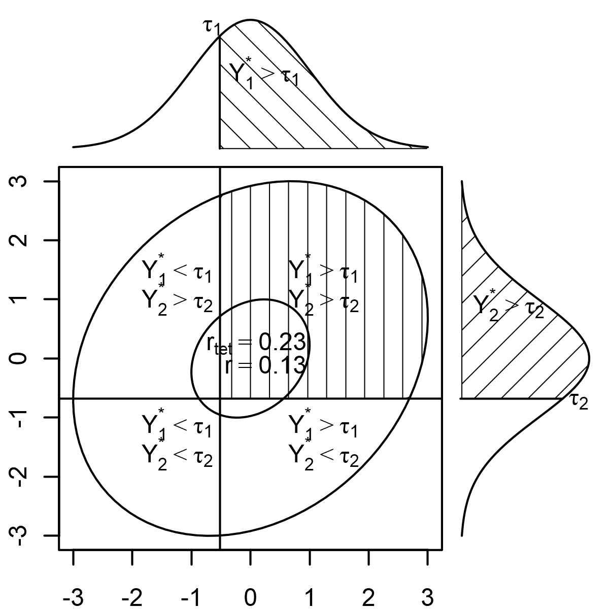
In the case of binary variables, such as true/false item responses, it is often hypothesized that the item responses \(Y_i\) are manifestations of an underlying normally distributed latent variable \(Y^{\star}_i\) and that the actual responses depend upon passing a fixed, yet unknown threshold \(\tau_i\). For a binary variable we have
\[ Y_i = 1 \iff Y^{\star}_i > \tau_i. \tag{3.1}\]
The tetrachoric correlation (Pearson, 1900) between the two binary variables \(Y_i\) and \(Y_j\) is then defined as the Pearson correlation coefficient between the two underlying latent variables \(Y^{\star}_i\) and \(Y^{\star}_j\),
\[ r_{\text{tet}_{Y_i Y_j}} = r_{Y^{\star}_i Y^{\star}_j}; \tag{3.2}\]
see Figure 3.1 for an illustration.
The distribution of scores in item \(i\) and item \(j\) is summarized in a contingency table (Table 3.1).
| \(Y_j = 0\) | \(Y_j = 1\) | ||
|---|---|---|---|
| \(Y_i = 0\) | \(n_{00}\) | \(n_{01}\) | \(n_{0 \bullet} = n_{00} + n_{01}\) |
| \(Y_i = 1\) | \(n_{10}\) | \(n_{11}\) | \(n_{1 \bullet} = n_{10} + n_{11}\) |
| \(n_{\bullet 0} = n_{00} + n_{01}\) | \(n_{\bullet 1} = n_{01} + n_{11}\) | \(n\) |
The thresholds \(\tau_i\) and \(\tau_j\) are calculated by enumerating the marginal empirical probability \(\hat{\pi}_{1 \bullet} = \frac{n_{1 \bullet}}{n} = \frac{1}{n} \sum_{p = 1}^{n} Y_{pi}\) for obtaining the score 1 in item \(i\), and the marginal empirical probability \(\hat{\pi}_{\bullet 1} = \frac{n_{\bullet 1}}{n} \frac{1}{n}\sum_{p = 1}^{n} Y_{pj}\) for obtaining the score 1 in item \(j\) as
\[ \tau_i = \Phi^{-1}(1 - \hat{\pi}_{1 \bullet}) \quad \text{and} \quad \tau_j = \Phi^{-1}(1 - \hat{\pi}_{\bullet 1}), \tag{3.3}\]
where \(\Phi^{-1}\) is the quantile function of the standard normal distribution, see Equation C.4 in Section 1.6.
The tetrachoric correlation \(r_{\text{tet}_{Y_i Y_j}}\) is then obtained by enumerating the joint empirical probability \(\hat{\pi}_{11} = \frac{n_{11}}{n} = \frac{1}{n}\sum_{p = 1}^{n} Y_{pi} Y_{pj}\) for obtaining 1 in both items and by using numerical optimizing algorithms to solve with respect to \(r_{\text{tet}_{Y_i Y_j}}\) the equation
\[ \hat{\pi}_{11} = \int_{\tau_i}^{\infty}\int_{\tau_j}^{\infty} \phi(y_i, y_j, r_{\text{tet}_{Y_i Y_j}}) \mathrm{d} y_j \mathrm{d} y_i, \tag{3.4}\]
where \(\phi\) is a density of the bivariate standard normal distribution.
Alternatively, the tetrachoric correlation may be approximated using the formula (Pearson, 1900):
\[ r_{\text{tet}_{Y_i Y_j}} \approx \cos\left(\frac{\pi}{1 + \sqrt{\frac{\hat{\pi}_{00}\hat{\pi}_{11}}{\hat{\pi}_{10}\hat{\pi}_{01}}}}\right), \tag{3.5}\]
where \(\pi \approx 3.14\) is the Euler constant, and \(\hat{\pi}_{00}\), \(\hat{\pi}_{01}\), \(\hat{\pi}_{10}\), and \(\hat{\pi}_{11}\) are the empirical joint probabilities obtained from the contingency Table 3.1 for scores from item \(i\) and item \(j\) by dividing its elements by \(n\).
The generalization of the tetrachoric correlation for the case of ordinal items with \(K_i +1\) categories \(k = 0, \dots, K_i\) is the polychoric correlation coefficient. The observed ordinal variables are once again assumed to dissect continuous normally distributed latent variables. Analogously to Equation 3.1, the item score is assumed to be \(Y_i = k\) in a case where the underlying latent variable falls between unobserved thresholds \(\tau_{i, k - 1} < Y^{\star}_i \leq \tau_{i, k}\), i.e,
\[ \begin{split} Y_i = 0 \iff &\ \quad \quad \ \ \ \, \ \ Y^{\star}_i \leq \tau_{i, 0},\\ Y_i = k \iff &\ \tau_{i, k - 1} < Y^{\star}_i \leq \tau_{i, k}, \quad k = 1, \dots, K_i, \end{split} \tag{3.6}\]
while \(\tau_{i, K_i} = \infty\).
The polychoric correlation coefficient between two ordinal items \(Y_i\) and \(Y_j\) is then defined by Equation 3.2, i.e., the Pearson correlation coefficient between the two underlying latent variables. The \(K_i\) and \(K_j\) thresholds are estimated using quantiles of the marginal empirical probabilities as in Equation 3.3, and the correlation coefficient is estimated from an equation similar to Equation 3.4. For further discussion on estimation of polychoric correlation, the reader is referred to Olsson (1979).
Tetrachoric correlation in the psych package. In R, tetrachoric correlation can be computed using the tetrachoric() function from the psych package, requiring a contingency table as an input, which can be obtained with the base table() function. The tetrachoric() function calculates the thresholds \(\tau_i\) and \(\tau_j\) using Equation 3.3, and it uses numerical optimizing and functions from the mnormt package to solve Equation 3.4 and to estimate the tetrachoric correlation coefficient.
As an example, we calculate the tetrachoric correlation coefficient between the first two items from the binary HCI dataset.
library(psych)
data(HCI, package = "ShinyItemAnalysis")
tetrachoric(table(HCI$"Item 1", HCI$"Item 2"))Call: tetrachoric(x = table(HCI$"Item 1", HCI$"Item 2"))
tetrachoric correlation
[1] 0.23
with tau of
0 0
-0.52 -0.68 The tetrachoric correlation coefficient between the first two items in the HCI dataset is 0.23. The latent scores needed to answer the two items correctly were estimated to be \(-0.52\) and \(-0.68\), i.e., \(0.52\) SD and \(0.68\) SD below average (latent) ability.
The graphical visualization of the calculation of this tetrachoric correlation coefficient, similar to Figure 3.1, may be obtained using the draw.tetra() function of the psych package:
draw.tetra(r = 0.23, t1 = -0.52, t2 = -0.68)The calculation of the thresholds \(\tau_1\) and \(\tau_2\) may be checked using Equation 3.3. We first calculate the contingency table (Table 3.1):
(tab <- table(HCI$"Item 1", HCI$"Item 2"))
      0   1
  0  66 130
  1  95 360
We then compute the joint empirical probabilities and the marginal empirical probabilities \(\hat{\pi}_{1 \bullet}\) and \(\hat{\pi}_{\bullet 1}\).
(ptab <- tab / sum(tab))
            0         1
  0 0.1013825 0.1996928
  1 0.1459293 0.5529954
(pi_1o <- sum(ptab[2, ]))[1] 0.6989247(pi_o1 <- sum(ptab[, 2]))[1] 0.7526882The qnorm() function is used to calculate the thresholds with Equation 3.3
qnorm(1 - pi_1o)[1] -0.5213104qnorm(1 - pi_o1)[1] -0.6829734The resulting thresholds of \(- 0.52\) and \(- 0.68\) match exactly those obtained from the tetrachoric() function.
We next calculate the approximate tetrachoric correlation using the formula Equation 3.5
cos(pi / (1 + sqrt(tab[1, 1] * tab[2, 2] / (tab[1, 2] * tab[2, 1]))))[1] 0.2519491The estimate of 0.25 is similar to the value of 0.23 obtained with the tetrachoric() function.
Polychoric correlation in the psych package. In R, the polychoric correlation can be computed using the polychoric() function from the psych package. For demonstration, we calculate the polychoric correlation between the first two items from the ordinal Anxiety dataset.
data(Anxiety, package = "ShinyItemAnalysis")
polychoric(table(Anxiety$R1, Anxiety$R2))
[1] "You seem to have a table, I will return just one correlation."$rho
[1] 0.8333789
$objective
[1] 1.558687
$tau.row
1 2 3 4
0.4608467 1.1583131 1.8433759 2.6068334
$tau.col
1 2 3 4
0.5236497 1.2897775 2.0104231 3.2147717 The polychoric correlation coefficient between the first two items, “I felt fearful” and “I felt frightened”, is 0.83. The latent anxiety needed to provide a response higher than 1, 2, 3, and 4 for item R1, i.e., to report feeling fearful more often than never, rarely, sometimes, and often, respectively, were estimated to be \(0.46\), \(1.16\), \(1.84\), and \(2.61\). Slightly higher levels of \(0.52\), \(1.29\), \(2.01\), and \(3.21\), respectively, were needed for item R2 to report feeling frightened more often than never, rarely, sometimes, and often, respectively.
Note that the polychoric correlation of binary variables is identical to the tetrachoric correlation. Correlation is now computed between all twenty items of the HCI dataset in order to explore the correlation structure of the test. We will calculate the tetrachoric correlations between the items using the polychoric() function from the psych package, and we will then save and display the values of the correlation matrix saved into the rho output.
(corHCI <- polychoric(x = HCI[, 1:20])$rho) Item 1 Item 2 Item 3 Item 4 Item 5 Item 6
Item 1 1.000000000 0.233800521 0.281749251 0.07068597 0.14244015 0.33702090
Item 2 0.233800521 1.000000000 0.479983532 0.12724753 0.21361261 0.13645093
Item 3 0.281749251 0.479983532 1.000000000 0.05081001 0.28433822 0.27341715
Item 4 0.070685967 0.127247530 0.050810011 1.00000000 0.11654649 0.08062829
Item 5 0.142440152 0.213612607 0.284338222 0.11654649 1.00000000 0.22118969
Item 6 0.337020899 0.136450930 0.273417148 0.08062829 0.22118969 1.00000000
Item 7 0.057576620 -0.024037196 0.067912846 0.01179921 0.11289096 0.14416090
Item 8 0.188556783 0.273458372 0.432704320 0.13388644 0.27065605 0.33521558
Item 9 0.111442699 0.009175606 0.081659415 0.42719489 0.09122704 0.07030200
Item 10 0.209169962 0.043857072 0.254144335 -0.01587917 0.19202019 0.32346509
Item 11 0.153151724 0.038679088 0.313614683 0.09662394 0.16772355 0.25943556
Item 12 0.320222559 0.150077282 0.271358370 0.15477419 0.15829109 0.40116977
Item 13 0.082415752 0.160900202 0.343565784 0.04153214 0.25020024 0.29350881
Item 14 0.314658597 0.123682697 0.269028730 0.08231158 0.23218880 0.24188109
Item 15 0.224006359 0.253804274 0.252037013 0.12240833 0.18718038 0.16693720
Item 16 0.288347435 0.277586233 0.294465424 0.16959229 0.26422010 0.30754644
Item 17 0.001387389 -0.045569778 0.006623588 0.10273401 0.04063115 0.02403374
Item 18 0.309245382 0.290492808 0.424508510 0.07540130 0.29931976 0.26923523
Item 19 0.214024597 0.149768334 0.362077749 0.03484372 0.20072586 0.27249273
Item 20 0.221532437 0.130287716 0.277272856 0.26483352 0.11726470 0.28265560
Item 7 Item 8 Item 9 Item 10 Item 11 Item 12
Item 1 0.057576620 0.18855678 0.111442699 0.20916996 0.15315172 0.32022256
Item 2 -0.024037196 0.27345837 0.009175606 0.04385707 0.03867909 0.15007728
Item 3 0.067912846 0.43270432 0.081659415 0.25414434 0.31361468 0.27135837
Item 4 0.011799206 0.13388644 0.427194892 -0.01587917 0.09662394 0.15477419
Item 5 0.112890957 0.27065605 0.091227040 0.19202019 0.16772355 0.15829109
Item 6 0.144160898 0.33521558 0.070301996 0.32346509 0.25943556 0.40116977
Item 7 1.000000000 0.12287068 0.106262355 -0.06035107 0.06177201 0.11843955
Item 8 0.122870676 1.00000000 0.081410412 0.14694942 0.23534520 0.17941735
Item 9 0.106262355 0.08141041 1.000000000 0.05478123 0.08428261 0.05402303
Item 10 -0.060351069 0.14694942 0.054781232 1.00000000 0.20693994 0.23070169
Item 11 0.061772012 0.23534520 0.084282608 0.20693994 1.00000000 0.32601031
Item 12 0.118439547 0.17941735 0.054023033 0.23070169 0.32601031 1.00000000
Item 13 0.004492976 0.23529660 0.075916765 0.32647627 0.35438550 0.24202683
Item 14 0.035465309 0.17511639 0.138875251 0.28892233 0.23730700 0.28119302
Item 15 0.038874319 0.17227537 0.067239450 0.25787596 0.18378312 0.18202104
Item 16 0.040229876 0.28623461 0.171468053 0.21108806 0.29011085 0.35297637
Item 17 0.038807499 -0.01383567 0.149868233 0.07099514 0.02542470 -0.04047666
Item 18 0.098159532 0.43904628 0.312632102 0.24698453 0.32626563 0.11858064
Item 19 0.229709032 0.34719832 0.197901058 0.22860078 0.30628858 0.28980752
Item 20 0.114722647 0.22468344 0.437050540 0.18466709 0.20514011 0.14681392
Item 13 Item 14 Item 15 Item 16 Item 17 Item 18
Item 1 0.082415752 0.31465860 0.22400636 0.28834743 0.001387389 0.30924538
Item 2 0.160900202 0.12368270 0.25380427 0.27758623 -0.045569778 0.29049281
Item 3 0.343565784 0.26902873 0.25203701 0.29446542 0.006623588 0.42450851
Item 4 0.041532144 0.08231158 0.12240833 0.16959229 0.102734005 0.07540130
Item 5 0.250200245 0.23218880 0.18718038 0.26422010 0.040631150 0.29931976
Item 6 0.293508810 0.24188109 0.16693720 0.30754644 0.024033739 0.26923523
Item 7 0.004492976 0.03546531 0.03887432 0.04022988 0.038807499 0.09815953
Item 8 0.235296603 0.17511639 0.17227537 0.28623461 -0.013835674 0.43904628
Item 9 0.075916765 0.13887525 0.06723945 0.17146805 0.149868233 0.31263210
Item 10 0.326476270 0.28892233 0.25787596 0.21108806 0.070995139 0.24698453
Item 11 0.354385496 0.23730700 0.18378312 0.29011085 0.025424703 0.32626563
Item 12 0.242026835 0.28119302 0.18202104 0.35297637 -0.040476656 0.11858064
Item 13 1.000000000 0.40672675 0.32286370 0.36865972 0.053371727 0.43033123
Item 14 0.406726746 1.00000000 0.34854413 0.22798644 -0.048777256 0.31977375
Item 15 0.322863701 0.34854413 1.00000000 0.27776255 0.037287947 0.31602530
Item 16 0.368659717 0.22798644 0.27776255 1.00000000 0.033521593 0.33938796
Item 17 0.053371727 -0.04877726 0.03728795 0.03352159 1.000000000 0.01791016
Item 18 0.430331228 0.31977375 0.31602530 0.33938796 0.017910163 1.00000000
Item 19 0.215389822 0.35349698 0.27119935 0.30176378 0.085191476 0.59437899
Item 20 0.333346688 0.41673780 0.19034667 0.23037753 0.008757819 0.34545844
Item 19 Item 20
Item 1 0.21402460 0.221532437
Item 2 0.14976833 0.130287716
Item 3 0.36207775 0.277272856
Item 4 0.03484372 0.264833516
Item 5 0.20072586 0.117264701
Item 6 0.27249273 0.282655603
Item 7 0.22970903 0.114722647
Item 8 0.34719832 0.224683443
Item 9 0.19790106 0.437050540
Item 10 0.22860078 0.184667088
Item 11 0.30628858 0.205140112
Item 12 0.28980752 0.146813915
Item 13 0.21538982 0.333346688
Item 14 0.35349698 0.416737797
Item 15 0.27119935 0.190346673
Item 16 0.30176378 0.230377526
Item 17 0.08519148 0.008757819
Item 18 0.59437899 0.345458441
Item 19 1.00000000 0.265469674
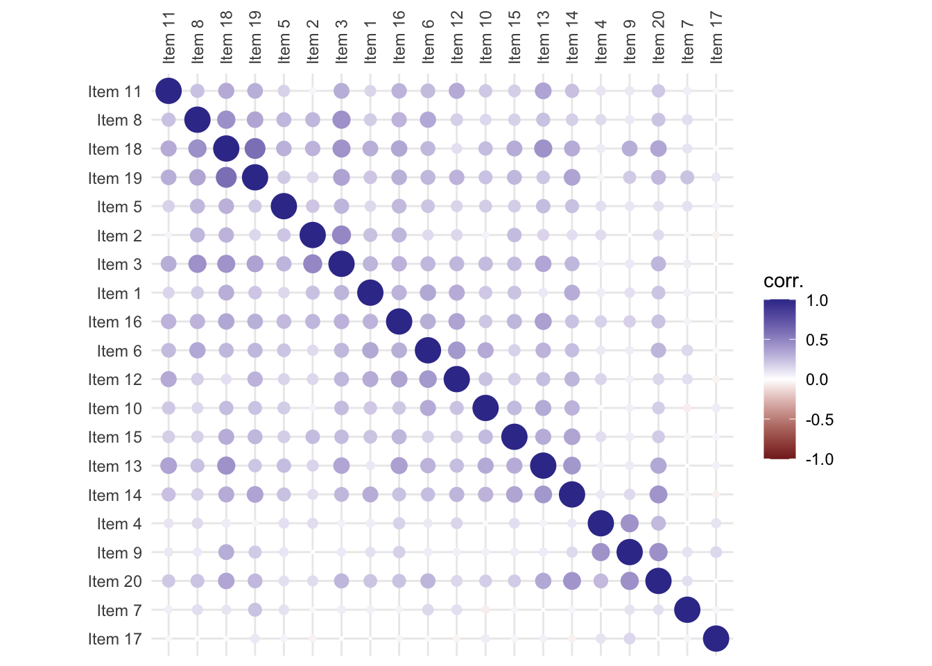
Item 20 0.26546967 1.000000000As expected, correlation between items 1 and 2 is again \(0.23\), as was earlier estimated with the tetrachoric() function. The correlation between item 4 and the other items seems to be rather low. The between-item correlations can be displayed with the plot_corr() function from the ShinyItemAnalysis package as a correlation heat map, with darker larger circles indicating stronger correlations (see Supplementary R code).
Tetrachoric and polychoric correlations in the lavaan package. The tetrachoric and polychoric correlations may also be calculated using the lavCor() function of the lavaan package. The function takes the original data frame or a lavaan object as an input, and it can return correlations, thresholds, as well as their standard errors and confidence intervals; see Supplementary R code.
A cluster analysis has found many uses in measurement and psychometrics. For example, in personality psychology, Cattell (1943) used cluster analysis for trait theory classification. The main aim of cluster analysis is to provide visual information about similarities and dissimilarities among objects. Classification has a long tradition in social sciences, and other fields as well. It may provide a reasoning behind the grouping of individuals into species or languages into language families, or may help by segmenting customers to allow for better targeting with advertisements. In the context of multi-item measurement, the objects may be either the respondents or the items. The latter (cluster analysis of items) can provide initial information about the internal structure of a test.
Two main steps of cluster analysis consist of
The first step involves specifying a distance matrix, which is an array with the distance between object \(i\) and \(j\) displayed in the \(i^{th}\) row and \(j^{th}\) column. The matrix is usually symmetric, because the distance does not depend upon the order of the objects. There are two main approaches for constructing the distance matrix: One is by estimating the distances directly, for example, by asking the respondents to judge the differences between objects. The other approach involves computing the distances from the data measured on the objects. For continuous data, the most commonly used distance measure is Euclidean distance. For measurements on two objects, the Euclidean distance can be interpreted as a straight line distance. In the context of continuous items \(i = 1, \dots, m\) measured on respondents \(p = 1, \dots, n,\) the Euclidean distance between items \(i_1\) and \(i_2\) is
\[ \delta_{i_1 i_2} = \sqrt{\sum_{p = 1}^n (X_{i_1p} - X_{i_2p})^2}. \]
Through the use of algebra, in continuous variables, the Euclidean distance can be shown to be equivalent to the measure of similarity based upon the Pearson correlation coefficient Equation 2.13 \(r_{i_1 i_2}\). This gives some reasoning to using \(1 - r_{i_1 i_2}\) as a distance between items \(i_1\) and \(i_2\).
The second step of cluster analysis involves using an algorithm for forming clusters. The most used methods are hierarchical clustering methods, either starting from a single item and subsequently creating clusters of similar items (agglomerative methods) or, alternatively, starting from a single cluster and splitting it into parts (divisive methods). We briefly describe some of the most common agglomerative clustering methods below.
The nearest neighbor method, also termed as the single linkage method, starts with single items as initial clusters. In the first step, items with the smallest distance between them are brought together into a cluster. In each subsequent step, after merging two items or clusters into a single one, the distance matrix is recalculated to reflect the distances between existing clusters and the newly created one. The nearest neighbor method defines the distance between clusters as the minimum distance between observations in one cluster and observations in the other clusters. The farthest neighbor method, on the other hand, uses the maximum distance between clusters. Similarly, the median linkage method calculates the distance as the median of the distance between an observation in one cluster and observation in another cluster. Based upon the selected method, in each step, the two clusters with the smallest distance between them are brought together into a cluster.
As an alternative to looking for pairs of clusters with the smallest distance between them, the Ward’s method (Ward, 1963), aims at merging the pair of clusters from all possible pairs by minimizing the within-cluster sum of squares. The algorithm again starts with single items as initial clusters. In each step, a pair of clusters is merged into a single cluster, involving the least loss of the information being measured by a sum of its squares. In other words, the aim of the method is to obtain the optimal value of an objective function, in this case the minimal variance. There are a number of other clustering methods available, including hierarchical, non-hierarchical, or model based. For more insight into cluster analysis, see Hennig et al. (2015).
Cluster analysis in R. We demonstrate the use of cluster analysis for information on between-item similarities in the HCI dataset. The cluster analysis is implemented within the base hclust() function. We must first compute the dissimilarities as 1 minus the polychoric correlation coefficient and save them in an appropriate format using the as.dist() function. Ward’s method is implemented by using the argument method = "ward.D2" and then is used to create hierarchical clusters of items. The clusters are displayed in the dendrogram using the ggdendrogram() function of the ggdendro package. (Figure 3.2).
hc <- hclust(d = as.dist(1 - corHCI), method = "ward.D2")
library(ggdendro)
ggdendrogram(data = hc)

library(ShinyItemAnalysis)
This is ShinyItemAnalysis version 1.5.5
- to run the interactive {shiny} app, call `run_app()`
- to learn more, visit `ShinyItemAnalysis.org`plot_corr(Data = HCI[, 1:20], cor = "polychoric", clust_method = "ward.D2")ℹ `n_clust = 0`, but the items will still be sorted according to `ward.D2` method.
• Set `clust_method = "none"` to keep the original order.Ignoring unknown labels:
• fill : "corr."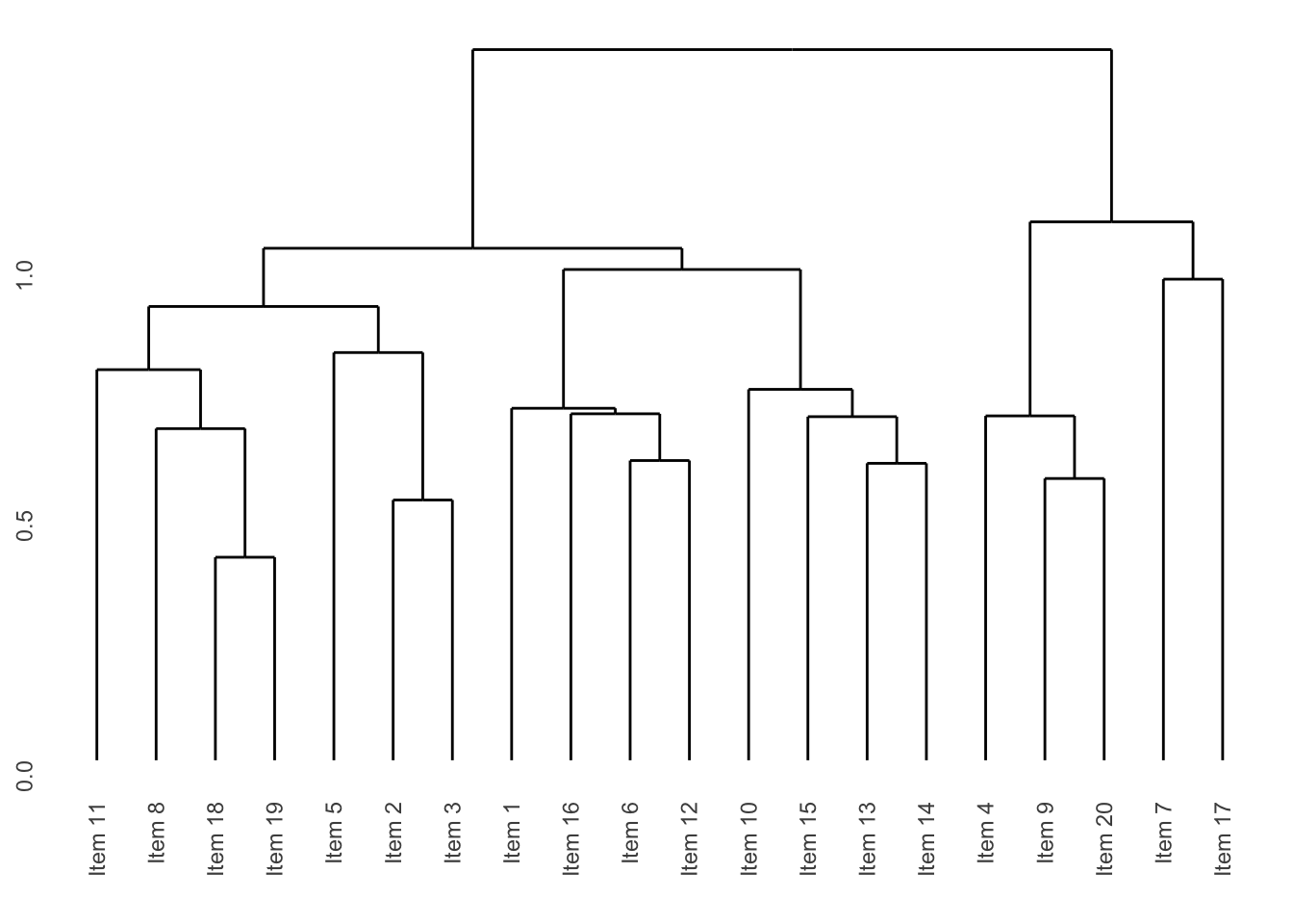
HCI dataset.
Clusters of correlated items need to be checked for content and other similarities to see if they are intentional. In the HCI dataset example, the cluster analysis (Figure 3.2 (a)) and also the internal structure displayed with the correlation heat map (Figure 3.2 (b)) point to three items of related content (items 4, 9, and 20) and two more difficult items with weaker correlation to other items (items 7 and 17). We will discuss these items more closely in Chapter 5.
Note that different clustering methods can lead to different clusters. If different clustering methods give the same clusters, this may point to some important aspect of the data structure.
Factor analysis (FA), pioneered by Spearman (1904), involves estimating unobserved, latent variables, also called factors. The aim is to explain between-item correlations by some small number of underlying factors. Confirmation of a factor model assumed by the theory may serve as a proof of validity based upon internal structure of the test. In psychometrics, the idea of latent variables is a central one, and it will be further discussed in Chapter 7 and Chapter 8 in the context of item response theory models.
We start with the assumption of a single latent factor \(\theta\), such as general quality of life, ability, or intelligence. Having \(m\) items \(i = 1, \dots, m\) (termed indicators or manifest variables in the context of the FA) measured on the respondents \(p = 1, \dots, n\), the single factor model assumes that
\[ Y_{pi} = \mu_i + \alpha_{i} \theta_p + \epsilon_{pi}, \tag{3.7}\]
where \(\mu_i\) is an intercept for the \(i^{\textrm{th}}\) indicator, \(\theta_p\) is the unobserved common factor of person \(p\), index \(\alpha_{i}\) is the factor loading for the \(i^{\textrm{th}}\) indicator describing the correlation between the indicator and latent factor, and \(\epsilon_{pi}\) is a random error. This equation is very similar to a simple linear regression model Equation 2.16 for item description; however, in Equation 3.7, the factor \(\theta_p\) is not observed. It is typically assumed that \(\theta_p\) and \(\epsilon_{pi}\) are independent, \(\text{E}(\theta_p) = 0\) and \(\text{Var}(\theta_p) = 1\), and that \(\epsilon_{pi}\) are unbiased, i.e., \(\text{E}(\epsilon_{pi}) = 0\), and independent; thus the item responses of single respondent \(Y_{p1}, \dots, Y_{pm}\) are conditionally independent given their ability/factor \(\theta_p\).
Using a vector notation, the latent variable model Equation 3.7 may be described as
\[ \boldsymbol{Y}_p = \boldsymbol{\mu} + \boldsymbol{\alpha} \theta_p + \boldsymbol{\epsilon}_p, \tag{3.8}\]
with \(\boldsymbol{Y}_p\) being the person’s \(p\) vector of observed indicators, \(\boldsymbol{\mu}\) the vector of indicator means, \(\boldsymbol{\alpha}\) the vector of common factor loadings, and \(\boldsymbol{\epsilon}_p\) the vector of uncorrelated random errors, all of length \(m\). Finally, \(\theta_p\) is the common factor (ability) of person \(p\) explaining the correlations between their observed indicators (item responses).
Using Equation 3.8 and the assumptions of the model, the true correlation matrix \(\mathbb{\Sigma}_{m \times m}\) is
\[ \mathbb{\Sigma} = \boldsymbol{\alpha}\boldsymbol{\alpha}^\top + \mathbb{\Psi}, \]
with \(\mathbb{\Psi}_{m \times m} = \text{E}(\boldsymbol{\epsilon}\boldsymbol{\epsilon}^\top)\) being a diagonal matrix, due to the assumed independence of residuals. The non-diagonal terms of the model-induced correlation matrix \(\mathbb{\Sigma}\) thus consist of terms \(\alpha_i \alpha_j\), i.e., products of the \(i^\textrm{th}\) and \(j^\textrm{th}\) item loading. Considering the diagonal of the model-induced correlation matrix \(\mathbb{\Sigma}\), the variance of the \(i^\textrm{th}\) scaled manifest variable, which is equal to 1, is partitioned into a portion accounted for by the common factor effect \(\alpha_i^2\), called the communality, and partly accounted for by the item residual variance, also called the “unique factor” effect, or the uniqueness, \(u^2_i = \text{E}(\epsilon_i \epsilon_i) = 1 - \alpha_i^2\).
Different estimation methods exist for the factor analytic model. One estimation method, the ordinary least-squares method, minimizes the squares of the elements in the residual matrix, i.e., the difference between the observed and the model-induced correlation matrix \(\mathbb{R} - \hat{\mathbb{\Sigma}}\). The residual matrix can also be used to describe the model fit and to make inferences. Note that the model parameters (factor loadings, communalities, uniqueness) can be simply estimated from the observed correlation matrix, and no additional information is needed. However, in order to make inferences, the number of respondents needs to be specified. Furthermore, the original observed scores on indicators (items, manifest variables) are needed in order to estimate the factor scores.
In the case of ordinal item scores \(Y_i\), these are assumed to be generated by an underlying continuous latent variable \(Y^{\star}_i\) as in Equation 3.6, which are then considered in the factor analytic model Equation 3.7. Correlations of the pairs of the unobserved continuous variables \(\text{Corr}(Y^{\star}_i, Y^{\star}_j)\) are estimated using the polychoric correlation matrix (see Section 3.2) and further used in an estimation of the model Equation 3.7.
Exploratory factor analysis in R. EFA can be performed in R with the base factanal() function, the fa() function from the psych package, and the efa() function from the lavaan package. To provide a practical demonstration, we shall consider the HCI dataset. We assume a single common factor, we use the ML estimation (using argument fm = "ml" in the fa() function), and we print the estimated factor loadings. The model can be fitted using solely the tetrachoric correlation matrix. Specifying the number of observations with argument n.obs = 651 allows for inferences.
library(psych)
fa(r = corHCI, nfactors = 1, fm = "ml")
Factor Analysis using method = ml
Call: fa(r = corHCI, nfactors = 1, fm = "ml")
Standardized loadings (pattern matrix) based upon correlation matrix
ML1 h2 u2 com
Item 1 0.44 0.197 0.80 1
Item 2 0.39 0.149 0.85 1
Item 3 0.61 0.378 0.62 1
Item 4 0.20 0.039 0.96 1
Item 5 0.42 0.173 0.83 1
Item 6 0.51 0.263 0.74 1
Item 7 0.15 0.023 0.98 1
Item 8 0.53 0.280 0.72 1
Item 9 0.28 0.080 0.92 1
Item 10 0.42 0.175 0.82 1
Item 11 0.48 0.227 0.77 1
Item 12 0.45 0.200 0.80 1
Item 13 0.57 0.319 0.68 1
Item 14 0.54 0.290 0.71 1
Item 15 0.46 0.212 0.79 1
Item 16 0.55 0.305 0.70 1
Item 17 0.04 0.002 1.00 1
Item 18 0.70 0.485 0.51 1
Item 19 0.61 0.368 0.63 1
Item 20 0.50 0.249 0.75 1
ML1
SS loadings 4.42
Proportion Var 0.22
Mean item complexity = 1
Test of the hypothesis that 1 factor is sufficient.
df null model = 190 with the objective function = 5.16
df of the model are 170 and the objective function was 1.91
The root mean square of the residuals (RMSR) is 0.05
The df corrected root mean square of the residuals is 0.06
Fit based upon off diagonal values = 0.95
Measures of factor score adequacy
ML1
Correlation of (regression) scores with factors 0.93
Multiple R square of scores with factors 0.86
Minimum correlation of possible factor scores 0.73fa(r = corHCI, nfactors = 1, fm = "ml", n.obs = 651)Factor Analysis using method = ml
Call: fa(r = corHCI, nfactors = 1, n.obs = 651, fm = "ml")
Standardized loadings (pattern matrix) based upon correlation matrix
ML1 h2 u2 com
Item 1 0.44 0.197 0.80 1
Item 2 0.39 0.149 0.85 1
Item 3 0.61 0.378 0.62 1
Item 4 0.20 0.039 0.96 1
Item 5 0.42 0.173 0.83 1
Item 6 0.51 0.263 0.74 1
Item 7 0.15 0.023 0.98 1
Item 8 0.53 0.280 0.72 1
Item 9 0.28 0.080 0.92 1
Item 10 0.42 0.175 0.82 1
Item 11 0.48 0.227 0.77 1
Item 12 0.45 0.200 0.80 1
Item 13 0.57 0.319 0.68 1
Item 14 0.54 0.290 0.71 1
Item 15 0.46 0.212 0.79 1
Item 16 0.55 0.305 0.70 1
Item 17 0.04 0.002 1.00 1
Item 18 0.70 0.485 0.51 1
Item 19 0.61 0.368 0.63 1
Item 20 0.50 0.249 0.75 1
ML1
SS loadings 4.42
Proportion Var 0.22
Mean item complexity = 1
Test of the hypothesis that 1 factor is sufficient.
df null model = 190 with the objective function = 5.16 with Chi Square = 3315.44
df of the model are 170 and the objective function was 1.91
The root mean square of the residuals (RMSR) is 0.05
The df corrected root mean square of the residuals is 0.06
The harmonic n.obs is 651 with the empirical chi square 691.6 with prob < 4.8e-64
The total n.obs was 651 with Likelihood Chi Square = 1226.23 with prob < 2.7e-159
Tucker Lewis Index of factoring reliability = 0.622
RMSEA index = 0.098 and the 90 % confidence intervals are 0.093 0.103
BIC = 124.88
Fit based upon off diagonal values = 0.95
Measures of factor score adequacy
ML1
Correlation of (regression) scores with factors 0.93
Multiple R square of scores with factors 0.86
Minimum correlation of possible factor scores 0.73The same output is provided when, alternatively, fitting the model by providing the original dataset with item responses and specifying the choice of the tetrachoric correlation matrix in argument cor. The advantage of providing the original data table is in the possibility to extract the factor scores, as we will demonstrate later.
FA1 <- fa(r = HCI[, 1:20], cor = "tetrachoric", nfactors = 1, fm = "ml")print(FA1$loadings, cutoff = 0)
Loadings:
        ML1
Item 1  0.444
Item 2  0.386
Item 3  0.615
Item 4  0.199
Item 5  0.416
Item 6  0.513
Item 7  0.152
Item 8  0.530
Item 9  0.283
Item 10 0.419
Item 11 0.476
Item 12 0.448
Item 13 0.565
Item 14 0.539
Item 15 0.460
Item 16 0.552
Item 17 0.045
Item 18 0.697
Item 19 0.607
Item 20 0.499

                 ML1
SS loadings    4.418
Proportion Var 0.221
The common factor is estimated to explain 22% of the variance. The item communalities can be extracted from the fitted model
FA1$communality Item 1 Item 2 Item 3 Item 4 Item 5 Item 6
0.197262317 0.149215874 0.378012966 0.039466865 0.173111800 0.263497382
Item 7 Item 8 Item 9 Item 10 Item 11 Item 12
0.023167428 0.280445568 0.080190064 0.175482793 0.226818151 0.200405522
Item 13 Item 14 Item 15 Item 16 Item 17 Item 18
0.319455796 0.290379702 0.211776760 0.304766627 0.002003481 0.485313094
Item 19 Item 20
0.367921168 0.248878074 which are simply squared item factor loadings as we demonstrate below for the first item:
FA1$loadings[1]^2[1] 0.1972623Item uniquenesses are complements of the communalities to 1:
FA1$uniquenesses Item 1 Item 2 Item 3 Item 4 Item 5 Item 6 Item 7 Item 8
0.8027377 0.8507841 0.6219870 0.9605331 0.8268882 0.7365026 0.9768326 0.7195544
Item 9 Item 10 Item 11 Item 12 Item 13 Item 14 Item 15 Item 16
0.9198099 0.8245172 0.7731818 0.7995945 0.6805442 0.7096203 0.7882232 0.6952334
Item 17 Item 18 Item 19 Item 20
0.9979965 0.5146869 0.6320788 0.7511219 To obtain the reproduced correlation matrix based upon the assumed model, the transposed loading vector cross-product \(\hat{\boldsymbol{\alpha}}\hat{\boldsymbol{\alpha}}^\top\) is obtained by using function tcrossprod() and added to the diagonal matrix, obtained with the diag() function, with item uniquenesses on the diagonal.
(HCI.rcor <- tcrossprod(loadings(FA1)) + diag(FA1$uniquenesses)) Item 1 Item 2 Item 3 Item 4 Item 5 Item 6
Item 1 1.00000000 0.17156535 0.27307089 0.088234490 0.18479295 0.22798707
Item 2 0.17156535 1.00000000 0.23749849 0.076740360 0.16072034 0.19828765
Item 3 0.27307089 0.23749849 1.00000000 0.122143304 0.25580951 0.31560327
Item 4 0.08823449 0.07674036 0.12214330 1.000000000 0.08265700 0.10197753
Item 5 0.18479295 0.16072034 0.25580951 0.082657003 1.00000000 0.21357553
Item 6 0.22798707 0.19828765 0.31560327 0.101977525 0.21357553 1.00000000
Item 7 0.06760222 0.05879582 0.09358199 0.030238151 0.06332894 0.07813166
Item 8 0.23520489 0.20456522 0.32559493 0.105206024 0.22033710 0.27183943
Item 9 0.12577153 0.10938752 0.17410596 0.056257003 0.11782125 0.14536118
Item 10 0.18605414 0.16181724 0.25755537 0.083221125 0.17429326 0.21503315
Item 11 0.21152464 0.18396975 0.29281428 0.094613960 0.19815372 0.24447083
Item 12 0.19882771 0.17292682 0.27523787 0.088934682 0.18625939 0.22979628
Item 13 0.25103105 0.21832974 0.34750314 0.112284989 0.23516285 0.29013060
Item 14 0.23933444 0.20815682 0.33131147 0.107053148 0.22420560 0.27661217
Item 15 0.20439074 0.17776517 0.28293879 0.091422999 0.19147077 0.23622579
Item 16 0.24519170 0.21325107 0.33941971 0.109673075 0.22969262 0.28338174
Item 17 0.01987992 0.01729021 0.02751984 0.008892194 0.01862327 0.02297634
Item 18 0.30940909 0.26910299 0.42831605 0.138397205 0.28985069 0.35760136
Item 19 0.26940115 0.23430680 0.37293293 0.120501847 0.25237174 0.31136195
Item 20 0.22157226 0.19270848 0.30672323 0.099108210 0.20756621 0.25608343
Item 7 Item 8 Item 9 Item 10 Item 11 Item 12
Item 1 0.067602223 0.23520489 0.12577153 0.18605414 0.21152464 0.19882771
Item 2 0.058795816 0.20456522 0.10938752 0.16181724 0.18396975 0.17292682
Item 3 0.093581986 0.32559493 0.17410596 0.25755537 0.29281428 0.27523787
Item 4 0.030238151 0.10520602 0.05625700 0.08322113 0.09461396 0.08893468
Item 5 0.063328944 0.22033710 0.11782125 0.17429326 0.19815372 0.18625939
Item 6 0.078131662 0.27183943 0.14536118 0.21503315 0.24447083 0.22979628
Item 7 1.000000000 0.08060523 0.04310218 0.06376116 0.07248995 0.06813869
Item 8 0.080605226 1.00000000 0.14996316 0.22184087 0.25221052 0.23707138
Item 9 0.043102175 0.14996316 1.00000000 0.11862536 0.13486498 0.12676960
Item 10 0.063761156 0.22184087 0.11862536 1.00000000 0.19950610 0.18753059
Item 11 0.072489952 0.25221052 0.13486498 0.19950610 1.00000000 0.21320321
Item 12 0.068138686 0.23707138 0.12676960 0.18753059 0.21320321 1.00000000
Item 13 0.086028886 0.29931582 0.16005368 0.23676781 0.26918093 0.25302313
Item 14 0.082020429 0.28536941 0.15259609 0.22573578 0.25663863 0.24123370
Item 15 0.070045148 0.24370444 0.13031651 0.19277753 0.21916846 0.20601270
Item 16 0.084027727 0.29235330 0.15633060 0.23126024 0.26291938 0.24713744
Item 17 0.006812893 0.02370374 0.01267514 0.01875037 0.02131727 0.02003768
Item 18 0.106035165 0.36892263 0.19727465 0.29182888 0.33177977 0.31186443
Item 19 0.092324358 0.32121933 0.17176618 0.25409414 0.28887921 0.27153901
Item 20 0.075933292 0.26419075 0.14127119 0.20898282 0.23759222 0.22333056
Item 13 Item 14 Item 15 Item 16 Item 17 Item 18
Item 1 0.25103105 0.23933444 0.20439074 0.24519170 0.019879923 0.30940909
Item 2 0.21832974 0.20815682 0.17776517 0.21325107 0.017290205 0.26910299
Item 3 0.34750314 0.33131147 0.28293879 0.33941971 0.027519845 0.42831605
Item 4 0.11228499 0.10705315 0.09142300 0.10967308 0.008892194 0.13839721
Item 5 0.23516285 0.22420560 0.19147077 0.22969262 0.018623271 0.28985069
Item 6 0.29013060 0.27661217 0.23622579 0.28338174 0.022976337 0.35760136
Item 7 0.08602889 0.08202043 0.07004515 0.08402773 0.006812893 0.10603516
Item 8 0.29931582 0.28536941 0.24370444 0.29235330 0.023703743 0.36892263
Item 9 0.16005368 0.15259609 0.13031651 0.15633060 0.012675144 0.19727465
Item 10 0.23676781 0.22573578 0.19277753 0.23126024 0.018750373 0.29182888
Item 11 0.26918093 0.25663863 0.21916846 0.26291938 0.021317268 0.33177977
Item 12 0.25302313 0.24123370 0.20601270 0.24713744 0.020037682 0.31186443
Item 13 1.00000000 0.30457098 0.26010251 0.31202478 0.025298689 0.39374621
Item 14 0.30457098 1.00000000 0.24798321 0.29748621 0.024119914 0.37539988
Item 15 0.26010251 0.24798321 1.00000000 0.25405214 0.020598319 0.32059013
Item 16 0.31202478 0.29748621 0.25405214 1.00000000 0.024710204 0.38458710
Item 17 0.02529869 0.02411991 0.02059832 0.02471020 1.000000000 0.03118198
Item 18 0.39374621 0.37539988 0.32059013 0.38458710 0.031181976 1.00000000
Item 19 0.34283312 0.32685905 0.27913644 0.33485832 0.027150012 0.42256001
Item 20 0.28196727 0.26882920 0.22957916 0.27540830 0.022329858 0.34753962
Item 19 Item 20
Item 1 0.26940115 0.22157226
Item 2 0.23430680 0.19270848
Item 3 0.37293293 0.30672323
Item 4 0.12050185 0.09910821
Item 5 0.25237174 0.20756621
Item 6 0.31136195 0.25608343
Item 7 0.09232436 0.07593329
Item 8 0.32121933 0.26419075
Item 9 0.17176618 0.14127119
Item 10 0.25409414 0.20898282
Item 11 0.28887921 0.23759222
Item 12 0.27153901 0.22333056
Item 13 0.34283312 0.28196727
Item 14 0.32685905 0.26882920
Item 15 0.27913644 0.22957916
Item 16 0.33485832 0.27540830
Item 17 0.02715001 0.02232986
Item 18 0.42256001 0.34753962
Item 19 1.00000000 0.30260124
Item 20 0.30260124 1.00000000The residual matrix can then be used to assess the fit of the model.
HCI.resid <- corHCI - HCI.rcorAnalogously, EFA can be performed with the base factanal() function with similar results (see Supplementary R code).
More generally, the indicators may describe a higher number \(Q\) of latent factors \(\theta_1, \dots, \theta_Q\). It is assumed that the number of factors is (much) smaller than the number of indicators, \(Q < m\). The single factor model Equation 3.7 is generalized to:
\[ Y_{pi} = \mu_i + \alpha_{i1} \theta_{p1} + \dots + \alpha_{iQ} \theta_{pQ} + \epsilon_{pi}. \tag{3.9}\]
Using a matrix notation, model Equation 3.9 can be described as
\[ \boldsymbol{Y}_p = \boldsymbol{\mu} + \mathbb{A} \boldsymbol{\theta}_p + \boldsymbol{\epsilon}_p, \tag{3.10}\]
analogously to Equation 3.8 but now with \(\boldsymbol{\theta}_{Q \times 1}\) being a vector of \(Q\) factor scores and \(\mathbb{A}_{m \times Q}\) being the matrix of \(Q\) factor loading vectors for each of the \(m\) indicators. The correlation matrix \(\mathbb{\Sigma}_{m \times m}\) is
\[ \mathbb{\Sigma} = \mathbb{A}\mathbb{\Phi}\mathbb{A}^\top + \mathbb{\Psi} \tag{3.11}\]
with \(\mathbb{\Psi}_{m \times m}\) diagonal matrix of uniquenesses, and \(\mathbb{\Phi}_{Q \times Q}\) factor correlation matrix. For estimation purposes, it is often assumed that the factors are orthogonal, which implies that \(\mathbb{\Phi}\) is an identity matrix and can be removed from Equation 3.11. This assumption can be further relaxed as we discuss in the next section.
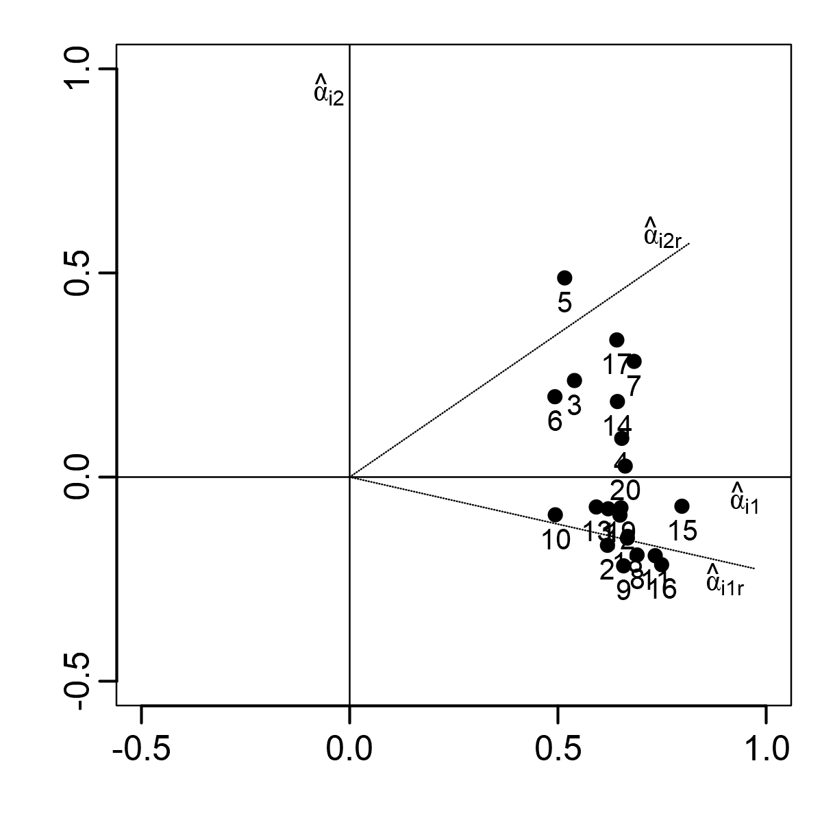
EFA with more factors in R. We illustrate this more general model by an example of the TestAnxietyCor dataset discussed in Bartholomew et al. (2008). The dataset contains the sample between-item correlations from responses of 335 male respondents to the test anxiety inventory. The inventory asked the respondents to report how often they experienced various symptoms of anxiety when taking tests including 1. lack of confidence, 2. uneasy, upset feeling, 3. thinking about grades, 4. freezing up, 5. thinking about getting through school, and others. We assume two factors, which are specified with an argument nfactors in the fa() function of the psych package. This time, we use default estimation based upon minimum residuals. A graphical interpretation of factor loadings in the two-factor solution is provided with the plot() method applied on the output of the fa() function (Figure 3.3 (a)).
data(TestAnxietyCor, package = "ShinyItemAnalysis")
(FA2_tAnxiety <- fa(r = TestAnxietyCor, nfactors = 2, n.obs = 335,
                    rotate = "none"))
Factor Analysis using method = minres
Call: fa(r = TestAnxietyCor, nfactors = 2, n.obs = 335, rotate = "none")
Standardized loadings (pattern matrix) based upon correlation matrix
MR1 MR2 h2 u2 com
i1 0.62 -0.08 0.39 0.61 1.0
i2 0.62 -0.17 0.41 0.59 1.1
i3 0.54 0.24 0.35 0.65 1.4
i4 0.65 0.09 0.44 0.56 1.0
i5 0.52 0.49 0.50 0.50 2.0
i6 0.49 0.20 0.28 0.72 1.3
i7 0.68 0.28 0.55 0.45 1.3
i8 0.69 -0.19 0.51 0.49 1.2
i9 0.66 -0.22 0.48 0.52 1.2
i10 0.49 -0.09 0.25 0.75 1.1
i11 0.73 -0.19 0.58 0.42 1.1
i12 0.65 -0.09 0.43 0.57 1.0
i13 0.59 -0.07 0.36 0.64 1.0
i14 0.64 0.19 0.45 0.55 1.2
i15 0.80 -0.07 0.64 0.36 1.0
i16 0.75 -0.21 0.61 0.39 1.2
i17 0.64 0.34 0.52 0.48 1.5
i18 0.67 -0.15 0.47 0.53 1.1
i19 0.65 -0.08 0.43 0.57 1.0
i20 0.66 0.03 0.44 0.56 1.0
MR1 MR2
SS loadings 8.25 0.83
Proportion Var 0.41 0.04
Cumulative Var 0.41 0.45
Proportion Explained 0.91 0.09
Cumulative Proportion 0.91 1.00
Mean item complexity = 1.2
Test of the hypothesis that 2 factors are sufficient.
df null model = 190 with the objective function = 9.5 with Chi Square = 3101.2
df of the model are 151 and the objective function was 0.89
The root mean square of the residuals (RMSR) is 0.03
The df corrected root mean square of the residuals is 0.03
The harmonic n.obs is 335 with the empirical chi square 90.84 with prob < 1
The total n.obs was 335 with Likelihood Chi Square = 287.9 with prob < 1.3e-10
Tucker Lewis Index of factoring reliability = 0.941
RMSEA index = 0.052 and the 90 % confidence intervals are 0.043 0.061
BIC = -590.03
Fit based upon off diagonal values = 1
Measures of factor score adequacy
MR1 MR2
Correlation of (regression) scores with factors 0.97 0.79
Multiple R square of scores with factors 0.94 0.62
Minimum correlation of possible factor scores 0.88 0.24In the output of the fa() function, MR1 and MR2 provide first and second factor loadings estimated using the minimum residuals method, h2 are communalities, i.e., the sum of squared factor loadings, and the u2 are the uniquenesses. From the first factor loadings MR1, we see that all items are positively correlated with the first factor, which can be interpreted as overall test anxiety. Interpretation of the second factor is not very clear. This necessitates the use of factor rotation.
There is in fact an infinite number of solutions to the minimization problem involved in the FA. This is because in Equation 3.11, the factor loadings can be rotated. Let’s first consider an orthogonal rotation in which the angle between the axes remains at \(90^{\circ}\). Geometrically this means that the axes are rotated. Algebraically, this means multiplying the factor loadings matrix \(\mathbb{A}_{m \times Q}\) and the original factors \(\boldsymbol{\theta}_{Q \times 1}\) by rotation matrix \(\mathbb{T}_{Q \times Q}\)
\[ \mathbb{A}_r = \mathbb{A} \mathbb{T} \, \, \, \, \, \boldsymbol{\theta}_r = \mathbb{T}^\top \boldsymbol{\theta}. \]
With orthogonal rotation, the rotation matrix \(\mathbb{T}\) is orthogonal, i.e., \(\mathbb{T}\mathbb{T}^\top = \mathbb{T}^\top\mathbb{T} = \mathbb{I};\) in other words, the rotation matrix does not need to be included in Equation 3.11, because \(\mathbb{T}\mathbb{\Phi}\mathbb{T}^\top = \mathbb{\Phi}_{Q \times Q}\).
Our goal is to obtain a simple structure, i.e., a situation in which the items have high loading on only one factor. If the theory supports that the two factors are correlated, then it is likely that no orthogonal rotation would provide a simple structure. In such a case, we can further consider oblique rotation, i.e., the rotation allowing for other than \(90^{\circ}\) angles between the axes of correlated factors.
Factor rotation in the psych package.
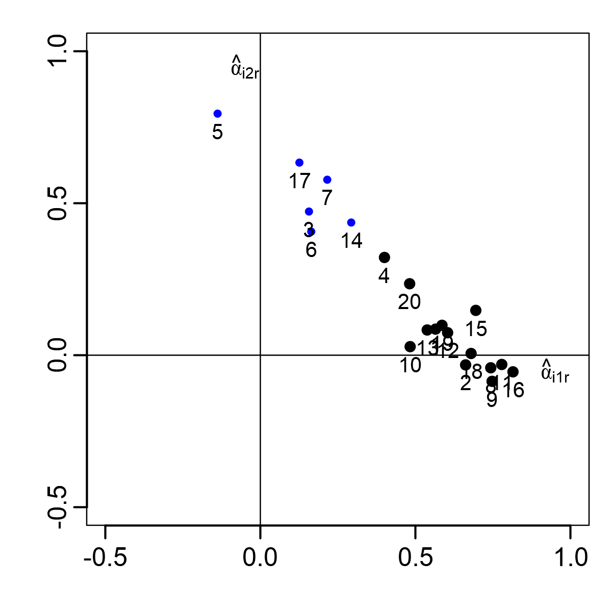
TestAnxietyCor dataset.
In the fa() function of the psych package, the rotation can be specified with an argument rotate, with "oblimin" being the default option. To print the loadings, we let only those values greater than 0.4 be printed while remembering that all items load on both factors. This is specified by argument cutoff = 0.4 of the print() method.
FA2_tAnxiety_obl <- fa(r = TestAnxietyCor, nfactors = 2, n.obs = 335,
                       rotate = "oblimin")
print(FA2_tAnxiety_obl$loadings, cutoff = 0.4)
Loadings:
    MR1    MR2
i1   0.565
i2   0.662
i3          0.473
i4   0.400
i5          0.795
i6          0.407
i7          0.578
i8   0.743
i9   0.747
i10  0.483
i11  0.779
i12  0.604
i13  0.538
i14         0.437
i15  0.695
i16  0.815
i17         0.634
i18  0.680
i19  0.586
i20  0.481

                 MR1   MR2
SS loadings    5.924 2.172
Proportion Var 0.296 0.109
Cumulative Var 0.296 0.405
With oblique rotation, interpretation of the two factors is now clearer: The first factor has high positive loading on items 1, 2, 4, (and other not displayed items), which can be interpreted as physiological reactions of the nervous system. The second factor has high loading on items 3, 5, and others, many of which involve the word “thinking”, which can be interpreted as psychological anxiety.
We use the plot() method to display the original and the rotated FA model (Figure 3.3). See Supplementary R code for further insight into the calculations involved in factor rotation.
Factor rotation in the GPArotation package. Another option for obtaining rotated factor solutions, besides the fa() function, is to use the rotations offered by the GPArotation package, by directly calling the respective argument in the base factanal() function. In the example below, we will first fit the two-factor model with the base factanal() function with no rotation and with the "oblimin" rotation. Alternatively, one can use the update() function on the output of the factanal() function while specifying the argument which is to be updated by rotation = "oblimin". The results are very similar to those obtained with the fa() function of the psych package (not printed here).
library(GPArotation)
Attaching package: 'GPArotation'The following objects are masked from 'package:psych':
equamax, variminFA2b_tAnxiety <- factanal(covmat = TestAnxietyCor, factors = 2,
rotation = "none", n.obs = 335)
FA2b_tAnxiety_obl <- factanal(covmat = TestAnxietyCor, factors = 2,
rotation = "oblimin", n.obs = 335)
update(FA2b_tAnxiety, rotation = "oblimin")
Call:
factanal(factors = 2, covmat = TestAnxietyCor, n.obs = 335, rotation = "oblimin")

Uniquenesses:
   i1    i2    i3    i4    i5    i6    i7    i8    i9   i10   i11   i12   i13
0.607 0.594 0.644 0.565 0.483 0.721 0.461 0.488 0.520 0.746 0.431 0.564 0.650
  i14   i15   i16   i17   i18   i19   i20
0.559 0.357 0.388 0.471 0.539 0.569 0.562

Loadings:
    Factor1 Factor2
i1   0.565
i2   0.660
i3   0.161   0.478
i4   0.417   0.305
i5  -0.132   0.799
i6   0.174   0.397
i7   0.229   0.563
i8   0.740
i9   0.749
i10  0.491
i11  0.771
i12  0.620
i13  0.527
i14  0.313   0.415
i15  0.708   0.132
i16  0.823
i17  0.143   0.625
i18  0.672
i19  0.586   0.101
i20  0.505   0.209

            Factor1 Factor2
SS loadings   6.494   2.588

Factor Correlations:
        Factor1 Factor2
Factor1   1.000   0.659
Factor2   0.659   1.000

Test of the hypothesis that 2 factors are sufficient.
The chi square statistic is 287.5 on 151 degrees of freedom.
The p-value is 1.47e-10 One of the goals or a potential by-product of the FA may be estimating the respondent’s level of unobserved latent trait(s); so-called factor scores. There is a number of methods used to compute the factor scores. The most common is a regression approach (Thurstone, 1947), which involves multiplying the inverted observed correlation matrix \(\mathbb{R}^{-1}_{m \times m}\) by the estimated factor loadings \(\widehat{\mathbb{A}}_{m \times Q}\) to find factor score coefficients (item weights) \(\widehat{\mathbb{B}}_{m \times Q}\) as
\[ \widehat{\mathbb{B}} = \mathbb{R}^{-1} \widehat{\mathbb{A}}. \tag{3.12}\]
These coefficients are then multiplied by the scaled input data scores (the matrix of Z scores) \(\mathbb{Z}_{n \times m}\) to obtain a matrix of estimated factor scores \(\widehat{\mathbb{F}}_{n \times Q}\):
\[ \widehat{\mathbb{F}} = \mathbb{Z} \widehat{\mathbb{B}}. \tag{3.13}\]
Factor scores in R. To provide a practical example, we return to the one factor model and the HCI dataset. In the code below, we use the base function solve() to invert the tetrachoric correlation matrix in order to compute the item weights, i.e. the factor score coefficients Equation 3.12. In the calculation of the factor scores according to Equation 3.13 we will then use the scale() function to compute the scaled input data \(\mathbb{Z}\).
(fscore.coef <- solve(corHCI) %*% FA1$loadings) ML1
Item 1 0.075394046
Item 2 0.061869529
Item 3 0.134697717
Item 4 0.028183363
Item 5 0.068565441
Item 6 0.094973476
Item 7 0.021232813
Item 8 0.100288080
Item 9 0.041951833
Item 10 0.069231887
Item 11 0.083935589
Item 12 0.076291063
Item 13 0.113171495
Item 14 0.103477493
Item 15 0.079557037
Item 16 0.108203550
Item 17 0.006111562
Item 18 0.184440473
Item 19 0.130765852
Item 20 0.090504892FSa <- scale(HCI[, 1:20]) %*% fscore.coef
head(FSa, n = 3) ML1
[1,] 0.8109138
[2,] 1.1816966
[3,] 0.8837516The same result is provided by using the factor.scores() function of the psych package with an argument method = "Thurstone". We will explicitly call the library psych here to avoid confusion with the function of the same name from the ltm package.
(FS <- psych::factor.scores(x = HCI[, 1:20], f = FA1, rho = corHCI,
method = "Thurstone"))$scores
ML1
[1,] 0.810913777
[2,] 1.181696613
[3,] 0.883751637
[4,] 1.224317129
[5,] 1.064316177
[6,] 1.224317129
[7,] 1.224317129
[8,] 0.431264924
[9,] 1.168324870
[10,] 0.926895148
[11,] 1.004095628
[12,] 0.724916657
[13,] 0.254552000
[14,] 0.028444232
[15,] 0.846342448
[16,] -1.320109805
[17,] -0.251103150
[18,] -0.187876597
[19,] 0.452119606
[20,] 0.001384171
[21,] -0.541000869
[22,] -0.053704763
[23,] 0.232417701
[24,] -0.557485359
[25,] -1.208881374
[26,] -0.297247603
[27,] -0.769719104
[28,] 0.611137520
[29,] -0.590110048
[30,] 0.395610830
[31,] -0.589508307
[32,] 0.109649155
[33,] 0.843533001
[34,] -0.227232452
[35,] -0.813979347
[36,] -0.776273371
[37,] -0.420307638
[38,] -0.433846655
[39,] -0.493744300
[40,] -1.228411858
[41,] 0.239400989
[42,] 0.074204711
[43,] -0.035403357
[44,] 0.785781839
[45,] -0.031295803
[46,] 1.153554061
[47,] 0.218206433
[48,] -0.373955597
[49,] -0.111469988
[50,] 0.725691777
[51,] 1.181696613
[52,] 0.363756241
[53,] 0.660721312
[54,] 0.526539466
[55,] -1.387856152
[56,] -0.023747768
[57,] -0.111538126
[58,] -1.234854129
[59,] 0.235183228
[60,] -0.360309045
[61,] 0.908955054
[62,] -0.119581339
[63,] -0.953602994
[64,] 0.780429827
[65,] -1.938648777
[66,] 1.013535245
[67,] 0.862106249
[68,] 0.686318559
[69,] 1.002971906
[70,] 0.730530910
[71,] -1.462426548
[72,] 1.015610037
[73,] 0.590742880
[74,] 0.343937181
[75,] 0.542129458
[76,] -0.606088503
[77,] -0.685136666
[78,] 0.220485090
[79,] 0.391870093
[80,] 0.121551944
[81,] 1.210945385
[82,] 1.068956006
[83,] 1.224317129
[84,] 0.592617258
[85,] 0.061178816
[86,] -1.541337293
[87,] 0.160680877
[88,] -0.288562418
[89,] 1.153554061
[90,] 0.547443115
[91,] -0.209773307
[92,] -0.185160127
[93,] -1.143878701
[94,] 0.308993655
[95,] 0.681332147
[96,] -0.731918505
[97,] 0.310889596
[98,] 0.544488558
[99,] 0.570362226
[100,] 0.076585971
[101,] 0.362585567
[102,] 0.216316197
[103,] 0.404877414
[104,] 0.842970954
[105,] -1.243064855
[106,] 0.993553109
[107,] 0.710927501
[108,] 0.616200586
[109,] 1.210945385
[110,] 1.168324870
[111,] -0.170250547
[112,] 0.895025651
[113,] 1.001775050
[114,] 0.908955054
[115,] 0.838534182
[116,] 0.520889634
[117,] -0.117466940
[118,] 0.186518270
[119,] 1.023454564
[120,] 0.173315962
[121,] 0.145128681
[122,] -0.494608144
[123,] 0.691655186
[124,] -0.450357039
[125,] -1.065597906
[126,] 0.325987769
[127,] 0.880476701
[128,] 0.045059344
[129,] 0.879706282
[130,] 0.331422239
[131,] -0.118786987
[132,] 0.221880716
[133,] 0.366047059
[134,] -0.683728925
[135,] -0.271004822
[136,] -0.517140944
[137,] 0.460883326
[138,] -0.472097760
[139,] 0.037377534
[140,] 0.051910167
[141,] -0.488731713
[142,] 0.275013432
[143,] 0.824285520
[144,] -0.919541185
[145,] -0.217760915
[146,] 0.178913993
[147,] -0.319140625
[148,] 0.154220794
[149,] 0.020065187
[150,] 0.656799092
[151,] 0.418990699
[152,] -1.512687254
[153,] -1.075776535
[154,] -1.376163995
[155,] 0.610628831
[156,] -0.443105839
[157,] -0.951009532
[158,] -0.384743184
[159,] 0.389071176
[160,] 1.083726815
[161,] 0.288432884
[162,] -0.892651721
[163,] 0.866906036
[164,] -0.280684853
[165,] -0.006088399
[166,] -0.115884431
[167,] 0.741446369
[168,] -0.525819990
[169,] -1.385077559
[170,] -0.303693065
[171,] 0.693174602
[172,] 0.086777305
[173,] -0.512390711
[174,] -0.601402089
[175,] 0.683071261
[176,] -0.982494621
[177,] 1.039707234
[178,] -0.105243438
[179,] -0.340761650
[180,] -0.134830213
[181,] -0.048848764
[182,] -0.299924399
[183,] -0.313366272
[184,] 1.015610037
[185,] 0.109536290
[186,] -0.736298270
[187,] 0.626587059
[188,] -0.123884160
[189,] -0.503289211
[190,] 0.405778660
[191,] 0.313608697
[192,] 0.522175938
[193,] 0.542739526
[194,] 0.667046244
[195,] 0.788951124
[196,] -1.440987615
[197,] -0.729670349
[198,] 0.612491190
[199,] 0.297641032
[200,] -0.465687385
[201,] -0.321005181
[202,] -1.535492467
[203,] -1.750761135
[204,] -0.065951595
[205,] 0.032523035
[206,] -0.080376085
[207,] 0.124282723
[208,] 0.618595796
[209,] 0.868664939
[210,] -0.387903408
[211,] 0.049231109
[212,] 0.351990772
[213,] -0.497127500
[214,] -0.584968577
[215,] 0.648900971
[216,] -0.651188685
[217,] -1.870599093
[218,] -1.255833994
[219,] -1.052617257
[220,] 0.442619407
[221,] -0.287958477
[222,] -1.631511123
[223,] 0.013869914
[224,] 0.674193253
[225,] -0.594427793
[226,] 0.130825083
[227,] -0.720339178
[228,] 1.126347331
[229,] 0.435453869
[230,] -1.311588945
[231,] -0.899160980
[232,] -0.818161564
[233,] -0.661437925
[234,] 0.641051189
[235,] 0.305198378
[236,] 0.234782073
[237,] -0.838730421
[238,] -0.843949578
[239,] -0.264570656
[240,] 0.339855018
[241,] -0.376909535
[242,] -1.311269658
[243,] -0.338492955
[244,] -1.287187616
[245,] -0.152619940
[246,] -0.620708355
[247,] 0.472963926
[248,] -0.324185636
[249,] -0.895729078
[250,] 0.031615418
[251,] -0.164222623
[252,] -0.320016243
[253,] 0.181683821
[254,] -1.179536091
[255,] -0.358849468
[256,] -1.675163455
[257,] -0.284983615
[258,] -0.308357427
[259,] -0.227533802
[260,] -0.681628011
[261,] -0.243180325
[262,] 0.648038020
[263,] -0.782441658
[264,] 0.347174277
[265,] -1.632498777
[266,] -0.098487287
[267,] 0.039916204
[268,] -0.471608321
[269,] 0.170786351
[270,] 0.536866640
[271,] -0.453294810
[272,] -0.580632591
[273,] -0.665957179
[274,] -0.203130526
[275,] 0.073945675
[276,] -0.044896273
[277,] -0.277023687
[278,] -0.518056782
[279,] -0.331789870
[280,] 0.506560333
[281,] -0.192213200
[282,] 0.136329308
[283,] -1.360426435
[284,] 0.220869763
[285,] 0.479481098
[286,] 0.233192239
[287,] -1.714569892
[288,] -1.375754556
[289,] 0.340766093
[290,] -0.434573510
[291,] -1.161845181
[292,] -1.781749022
[293,] 0.914841321
[294,] 1.012811119
[295,] 0.712791351
[296,] 0.572560875
[297,] 0.812988569
[298,] -0.054801821
[299,] -0.539651133
[300,] 0.762142911
[301,] -1.145549961
[302,] -0.340873018
[303,] -1.082434470
[304,] -0.209681295
[305,] 0.316322350
[306,] -0.909656366
[307,] 0.343638530
[308,] -0.878183138
[309,] -1.528786172
[310,] -0.867001350
[311,] 0.500603887
[312,] -1.261506500
[313,] -2.001277059
[314,] 0.856150325
[315,] -0.127793166
[316,] -1.050540298
[317,] -1.869100887
[318,] 0.482881992
[319,] -1.177734552
[320,] -1.828760291
[321,] 1.139719074
[322,] 0.606880142
[323,] -0.221900845
[324,] -0.597131865
[325,] -1.049621342
[326,] 0.745102415
[327,] -0.972492073
[328,] -1.956507112
[329,] -1.339399317
[330,] -0.454685801
[331,] 0.776897297
[332,] -0.356539033
[333,] -0.182838494
[334,] 0.351215652
[335,] -0.225675112
[336,] -0.615304849
[337,] 0.505754199
[338,] -0.651195367
[339,] -0.240714777
[340,] 1.068956006
[341,] -0.515334494
[342,] 1.081028078
[343,] 1.110933545
[344,] 0.381390368
[345,] 0.892601459
[346,] 0.693245020
[347,] 0.577004509
[348,] -0.150247027
[349,] -0.549507673
[350,] 0.687609832
[351,] 1.013535245
[352,] 0.570719963
[353,] 0.161001934
[354,] 0.432687824
[355,] -0.825758253
[356,] -1.222306067
[357,] 0.624997226
[358,] -0.301008575
[359,] 0.003105232
[360,] -0.667418372
[361,] -0.478370626
[362,] 0.131392374
[363,] -0.330484641
[364,] 0.585672961
[365,] -0.440140019
[366,] 0.678856020
[367,] -0.068148526
[368,] -1.137564283
[369,] 0.517706984
[370,] 0.478576980
[371,] 0.144723204
[372,] 0.932208839
[373,] 0.324789938
[374,] 0.737575388
[375,] 0.766605875
[376,] 0.943084053
[377,] 0.208890576
[378,] 0.608552549
[379,] 0.882036683
[380,] 0.981016238
[381,] 1.110933545
[382,] 0.875591220
[383,] 0.465356111
[384,] -0.938631036
[385,] 0.449387659
[386,] -0.156587838
[387,] 1.110933545
[388,] 0.091391583
[389,] -0.057485153
[390,] 0.867104958
[391,] 0.663572387
[392,] 1.030380845
[393,] -0.873424379
[394,] 0.250195858
[395,] -0.034818373
[396,] 1.153554061
[397,] 0.089644762
[398,] 0.749760275
[399,] 0.562446319
[400,] -0.481080556
[401,] 0.984286472
[402,] 0.358141934
[403,] -0.777185928
[404,] 0.826960755
[405,] -0.038757089
[406,] -1.026951862
[407,] 0.291101378
[408,] -1.853672457
[409,] 0.577218270
[410,] -0.305708606
[411,] 0.342682351
[412,] -0.720183654
[413,] -0.600145243
[414,] -1.027254641
[415,] 0.377898403
[416,] -0.261325168
[417,] 0.622093838
[418,] 1.068956006
[419,] -1.397420341
[420,] 1.068956006
[421,] 0.564007443
[422,] 0.444880438
[423,] 0.868664939
[424,] 0.577217127
[425,] 0.670369757
[426,] 0.570569457
[427,] 0.429145582
[428,] 0.080955279
[429,] -0.387233404
[430,] 0.655835832
[431,] 0.426367471
[432,] -0.552515943
[433,] 0.562446319
[434,] 0.711361979
[435,] -1.169731262
[436,] 0.523065608
[437,] 0.708326615
[438,] 0.761437714
[439,] -1.300567458
[440,] 0.176122395
[441,] 0.091561694
[442,] 0.603502344
[443,] 0.420122215
[444,] 0.670258659
[445,] 0.804364909
[446,] 0.484079866
[447,] 0.144956892
[448,] 1.097098558
[449,] 0.766782741
[450,] -0.175412413
[451,] -1.258488090
[452,] 0.045504048
[453,] 0.463297062
[454,] 0.481331572
[455,] -0.244038290
[456,] 0.670177577
[457,] 0.010588652
[458,] 1.126347331
[459,] 0.594055756
[460,] 0.872220806
[461,] 0.347329800
[462,] -0.435113535
[463,] -0.145216687
[464,] 0.884917609
[465,] 0.230917562
[466,] 1.015610037
[467,] 0.495428337
[468,] 0.129556474
[469,] 0.526539466
[470,] 0.442524991
[471,] -0.973182560
[472,] 0.380122876
[473,] 0.510718443
[474,] -0.139422614
[475,] -0.792618790
[476,] 0.470549701
[477,] 0.769971016
[478,] 0.704353069
[479,] 0.111376284
[480,] 0.650200643
[481,] -0.706953308
[482,] 0.388852907
[483,] 0.402445367
[484,] 0.572159290
[485,] 0.516704388
[486,] 0.352255667
[487,] -0.378800020
[488,] 0.771011030
[489,] 0.497492671
[490,] 0.913000409
[491,] 0.926372152
[492,] 0.472767436
[493,] -1.702796706
[494,] 0.266529168
[495,] 0.118849179
[496,] 0.195554400
[497,] -0.179090225
[498,] 0.818199896
[499,] 0.888962964
[500,] 0.448349595
[501,] 0.491900106
[502,] -0.969606414
[503,] -0.094096035
[504,] 0.824484442
[505,] -0.154503895
[506,] 0.123484676
[507,] -0.301978702
[508,] 0.092981416
[509,] 0.729160933
[510,] 0.867104958
[511,] 0.925666955
[512,] -1.310078285
[513,] 0.670170835
[514,] 0.693768016
[515,] -0.612559298
[516,] 0.577533016
[517,] 0.888391466
[518,] 0.888391466
[519,] 0.734276781
[520,] 0.888391466
[521,] -0.683115240
[522,] 0.888391466
[523,] 0.828925350
[524,] 0.745102415
[525,] 0.106117159
[526,] 0.328540065
[527,] 0.282201617
[528,] 0.419391788
[529,] 0.462759403
[530,] 0.170786351
[531,] 0.543150108
[532,] 0.517456002
[533,] 0.689199665
[534,] 0.884300197
[535,] 1.181696613
[536,] 0.677456954
[537,] -0.084837000
[538,] 0.658198944
[539,] 1.126347331
[540,] -0.580485645
[541,] 1.026335491
[542,] -0.673439005
[543,] 0.074484221
[544,] 0.547990612
[545,] 1.224317129
[546,] -0.489473757
[547,] 0.686540418
[548,] 0.925666955
[549,] 0.249880714
[550,] -0.574211970
[551,] -0.520521491
[552,] -0.712899475
[553,] 1.068956006
[554,] -0.009787435
[555,] -0.262423631
[556,] 0.951703012
[557,] -1.674866688
[558,] 0.086714913
[559,] 0.597257088
[560,] 0.189743701
[561,] 0.322113219
[562,] -0.746414337
[563,] 0.810913777
[564,] -0.715244990
[565,] -1.231031129
[566,] -0.840021087
[567,] 0.627721979
[568,] 0.627721979
[569,] -0.945063002
[570,] -2.064342606
[571,] -1.408804850
[572,] -1.273587384
[573,] -0.204266787
[574,] -1.424647612
[575,] -1.114391870
[576,] 0.970914729
[577,] -0.390346004
[578,] 0.825055940
[579,] -2.014602947
[580,] -0.426384707
[581,] 0.094870629
[582,] -0.415559739
[583,] -0.847760868
[584,] -1.589011665
[585,] -1.027590247
[586,] -1.467100416
[587,] -0.439458257
[588,] 0.467751346
[589,] -0.669285151
[590,] 0.074891702
[591,] 0.368967568
[592,] 0.574847327
[593,] 0.254171797
[594,] -1.329113955
[595,] 0.591518226
[596,] -1.025270304
[597,] -0.622123460
[598,] -0.848695668
[599,] 0.711361979
[600,] 0.592858900
[601,] 0.168149677
[602,] 0.011420579
[603,] -0.424666024
[604,] -0.738190251
[605,] 0.744767598
[606,] -0.049219607
[607,] -0.575619587
[608,] 0.644989316
[609,] 0.025685787
[610,] -0.395949210
[611,] -0.219441754
[612,] -0.287269985
[613,] -0.225428059
[614,] 0.438077221
[615,] -0.550745665
[616,] -0.487268220
[617,] 0.114820940
[618,] -1.008223360
[619,] -1.087201644
[620,] -0.864934309
[621,] -0.633405504
[622,] 0.198140982
[623,] -0.102332833
[624,] -0.913347786
[625,] -1.435009264
[626,] -0.064234923
[627,] 0.311086897
[628,] 1.168324870
[629,] -0.798828292
[630,] 0.717431181
[631,] 1.013535245
[632,] -1.460876887
[633,] -1.707277924
[634,] -0.503873891
[635,] 0.771552270
[636,] -0.424372762
[637,] -1.613455778
[638,] 0.124536338
[639,] -0.558406277
[640,] -0.821362547
[641,] -0.588759013
[642,] -1.014864693
[643,] 0.706882147
[644,] -0.240875873
[645,] -0.316228952
[646,] -1.603680447
[647,] -0.749500719
[648,] 0.037706626
[649,] -1.381798728
[650,] -0.769772018
[651,] 0.132523704
$weights
                ML1
Item 1  0.075394046
Item 2  0.061869529
Item 3  0.134697717
Item 4  0.028183363
Item 5  0.068565441
Item 6  0.094973476
Item 7  0.021232813
Item 8  0.100288080
Item 9  0.041951833
Item 10 0.069231887
Item 11 0.083935589
Item 12 0.076291063
Item 13 0.113171495
Item 14 0.103477493
Item 15 0.079557037
Item 16 0.108203550
Item 17 0.006111562
Item 18 0.184440473
Item 19 0.130765852
Item 20 0.090504892
$r.scores
ML1
ML1 1
$missing
[1] FALSE
$R2
ML1
0.8637337 The item score of the fourth item was only 0.03, while it was 0.13 for the third item. The first respondent had ability estimated at 0.81 SD above the mean, while the second respondent had ability of 1.18 SD above the mean.
In the lavaan package, the factor scores can be extracted using the predict() or lavPredict() functions; see Supplementary R code for examples.
Until now, we have assumed that the number of factors is known. However, an important aspect of the EFA is to determine the optimal number of factors. There are several strategies which may be used for this task. Perhaps the most important one is interpretability. In the case of the HCI dataset, this instrument is supposed to measure a single underlying trait, that is, understanding the concept of homeostasis; thus the best interpretability is achieved with a single factor. In the case of the TestAnxietyCor dataset, an additional factor may provide an extra interpretation. We will now describe various approaches to assess the optimal number of factors based upon data.
The classical approach is to carry out a principal component analysis (PCA), because the number of components needed is normally a good estimate for the number of factors (Fabrigar et al., 1999). The PCA involves the eigenvalue decomposition of the data correlation matrix \(\mathbb{R}\) with dimension \(m \times m\). That is, finding diagonal matrix \(\mathbb{\Lambda}_{m \times m}\), containing the eigenvalues \(\lambda_1 \geq \dots \geq \lambda_m\) on the diagonal, and an orthogonal matrix \(\mathbb{U}_{m \times m}\) containing the eigenvectors, such that
\[ \mathbb{R} = \mathbb{U} \mathbb{\Lambda} \mathbb{U}^{-1}. \]
The eigenvalues are the variances of the components. The variance of \(m\) standardized items is \(m\); thus the sum of all eigenvalues is \(m\).
Eigenvalues and Eigenvectors in R. In R, the eigenvalues can be extracted with argument values of the base function eigen(). They can also be extracted with argument e.values as the output of the model fitted with the fa() function in the psych package. We will demonstrate the calculation using the TestAnxietyCor dataset.
eigen(TestAnxietyCor)$values [1] 8.7790483 1.3495197 0.9710369 0.8880112 0.7744172 0.7416370 0.7062043
[8] 0.6548784 0.5706527 0.5434893 0.5409148 0.5059961 0.4720353 0.4359095
[15] 0.4189898 0.3773801 0.3482704 0.3324050 0.3138215 0.2753824The eigenvalues can be used to decide the optimal number of factors in several ways: The Kaiser rule (Kaiser, 1960) suggests discarding all components below the eigenvalue of 1 (the variance of a single item). Thus in the example of the TestAnxietyCor dataset, when considering the Kaiser rule, we would retain 2 factors.
The scree test (Cattell, 1966) suggests plotting the eigenvalues against the component or factor number (a scree plot) and to look for an “elbow”, that is, a point after which the decrease of the eigenvalues is slower and resembles a “scree”.
A more sophisticated method called a parallel analysis (Horn, 1965) involves generating simulated uncorrelated random data of the same size and comparing the eigenvalues of the original data to the eigenvalues generated from the simulated matrix. The number of factors with the eigenvalue larger than the eigenvalue at the first (leftmost) curves crossing is then the optimal number to extract in the FA.
Scree plot and parallel analysis in R. In R, a scree plot can be created using the scree() function of the psych package. A parallel analysis is implemented in the fa.parallel() function of the psych package, and the fa_parallel() function of the ShinyItemAnalysis package, which is also used within the interactive application. We will use the latter one for demonstration.
library(ShinyItemAnalysis)
fa_parallel(Data = TestAnxietyCor, n_obs = 335, method = "pca")
The input was recognized as a correlation matrix.
Assuming 335 observations in the original data.Warning: Using `size` aesthetic for lines was deprecated in ggplot2 3.4.0.
ℹ Please use `linewidth` instead.
ℹ The deprecated feature was likely used in the ShinyItemAnalysis package.
Please report the issue at
<https://github.com/patriciamar/ShinyItemAnalysis/issues>.According to the parallel analysis, the optimal number of principal components is 1.
Following the Kaiser rule, 2 components are recommended.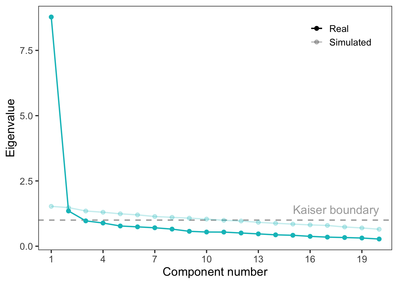
TestAnxietyCor dataset.
In the TestAnxietyCor dataset, the scree plot may suggest using two components; however, the parallel analysis suggests one component may be enough (Figure 3.4).
Note that the different procedures can imply a different number of factors. The final recommendation is to retain factors until they can be interpreted. In the TestAnxietyCor dataset, this would lead us to the two factors that we discussed earlier.
To assess goodness of fit and to select between two or more competing models, the fit indices, such as the AIC Equation 2.30 and BIC Equation 2.31, presented in Chapter 2, may be used.
In the context of FA, popular alternatives include the \(\chi^2\) goodness-of-fit test based on likelihood, and corresponding fit indices. The goodness-of-fit \(\chi^2\) test uses the likelihood, which in this case is based on the differences between the observed and model-induced covariance matrices.
The \(\chi^2\) statistic has asymptotically a \(\chi^2\) distribution Equation C.5 with degrees of freedom equal to the number of values from the variance/covariance matrix minus the number of estimated parameters (i.e., factor loadings, residual variances, unfixed variances, and covariances of the factors). The test may also be used to directly compare two nested models.
Besides formal statistical tests, several fit indices were developed to assess model fit and to compare competing models (Bentler & Bonett, 1980; Hu & Bentler, 1999). The root mean square error of approximation (RMSEA) is defined as
\[ \text{RMSEA} = \frac{\chi^2 - \text{df}}{\text{df} \cdot (n - 1)}. \tag{3.14}\]
Recall that under the \(\chi^2\) distribution, the expected value of the statistic is equal to the degrees of freedom, df. Smaller values of RMSEA close to 0 thus indicate better model fit. According to the rules of thumb, values \(\leq 0.05\) are indicative of close fit, values \(< 0.10\) indicate acceptable fit, while values \(\geq 0.10\) are indicative of poor fit.
While the RMSEA is an absolute measure of fit, the following two fit indices are relative fit measures, because they compare the performance of the model of interest (the target model \(T\)) to a baseline (null) model \(B\), in which all covariances are set to zero and the variances are freely estimated. The comparative fit index (CFI) is defined as
\[ \text{CFI} = \frac{(\chi^2_B - \text{df}_B) - (\chi^2_T - \text{df}_T)}{(\chi^2_B - \text{df}_B)}. \tag{3.15}\]
If the target model is correctly specified, then \((\chi^2_T - \text{df}_T)\) is close to 0 and CFI is close to 1. Values \(\geq 0.90\), or conservatively \(\geq 0.95\), are claimed as indicative of good fit.
The Tucker-Lewis index (TLI) is another relative or incremental fit index. The TLI uses a relative chi-square, also called normed chi-square \(\frac{\chi^2}{df}\). The TLI compares the relative chi-square of the target model with the one of the baseline (null) model as follows:
\[ \text{TLI} = \frac{\frac{\chi^2_B}{\text{df}_B} - \frac{\chi^2_T}{\text{df}_T}}{\frac{\chi^2_B}{\text{df}_B} - 1}. \tag{3.16}\]
If the target model is correctly specified then value of the relative chi-square \(\frac{\chi^2}{\text{df}_T}\) is close to 1 and TLI is close to 1. As for the CFI, the values \(\geq 0.90\), or conservatively \(\geq 0.95\), are claimed as indicative of good fit.
In previous sections, we described the EFA, which did not pose any assumptions on the number of factors or internal structure. In the fitted EFA models, all items are loaded on all of the factors, even though some of the loadings were small. In this section, we will describe confirmatory factor analysis (CFA), which is used in cases when a hypothesis about the internal structure exists and needs to be confirmed. The hypothesis which is being evaluated states that certain indicators will load only on certain factors. This model is similar to the model Equation 3.10; however, additional restrictions are put on the factor loading matrix \(\mathbb{A}\), whereby some elements are set at 0.
Confirmatory factor analysis in the lavaan package. In R, the CFA can be implemented with the lavaan package, which allows for more general latent variable analysis. We will demonstrate the CFA on an example of the BFI2 dataset.
data(BFI2, package = "ShinyItemAnalysis")
head(BFI2, n = 2)
i1 i2 i3 i4 i5 i6 i7 i8 i9 i10 i11 i12 i13 i14 i15 i16 i17 i18 i19 i20 i21
1 5 5 2 3 5 4 4 3 4 5 5 4 3 4 2 3 5 3 2 5 4
2 4 5 4 3 3 3 5 3 2 4 4 2 4 2 3 4 5 4 3 4 4
i22 i23 i24 i25 i26 i27 i28 i29 i30 i31 i32 i33 i34 i35 i36 i37 i38 i39 i40
1 4 4 3 5 4 4 5 5 5 3 5 4 4 5 4 3 4 2 4
2 4 4 2 2 4 2 4 3 4 5 5 5 4 5 3 4 4 1 4
i41 i42 i43 i44 i45 i46 i47 i48 i49 i50 i51 i52 i53 i54 i55 i56 i57 i58 i59
1 4 5 5 4 5 4 2 2 2 5 4 5 5 2 5 5 5 1 4
2 4 3 4 2 4 4 4 5 2 4 4 5 4 1 4 4 3 3 2
i60 Gender Age Educ
1 2 0 21 NA
2 3 0 25 NAThe BFI2 contains 60 items measuring personality in five domains: Extraversion, Agreeableness, Open-Mindedness, Conscientiousness, and Negative Emotionality. Each item is hypothesized to load on one of the five domains, and some correlations are expected between the domains. While all 60 items and all five domains were analyzed in the original paper, for the purpose of this demonstration, we will use only two domains (Extraversion and Negative Emotionality), with a reduced dataset consisting of only the 24 items loading on these two factors.
We first need to define the model by specifying which items load on which factor. We will specify the names of hypothesized factors (E and N), and using the =~ operator, we will declare by which items these factors are manifested.
model_EN <- 'E =~ i1 + i6 + i11 + i16 + i21 + i26 +
                  i31 + i36 + i41 + i46 + i51 + i56
             N =~ i4 + i9 + i14 + i19 + i24 + i29 +
                  i34 + i39 + i44 + i49 + i54 + i59'
The CFA model is then fitted using the cfa() function of the lavaan package by specifying the model and the data.
library(lavaan)This is lavaan 0.6-21
lavaan is FREE software! Please report any bugs.
Attaching package: 'lavaan'The following object is masked from 'package:psych':
cor2covfit_EN <- cfa(model_EN, data = BFI2)An overview for the specification of estimated parameters is provided using the parTable() method.
parTable(fit_EN) id lhs op rhs user block group free ustart exo label plabel start est
1 1 E =~ i1 1 1 1 0 1 0 .p1. 1.000 1.000
2 2 E =~ i6 1 1 1 1 NA 0 .p2. 0.813 0.969
3 3 E =~ i11 1 1 1 2 NA 0 .p3. 0.453 0.470
4 4 E =~ i16 1 1 1 3 NA 0 .p4. 1.413 1.420
5 5 E =~ i21 1 1 1 4 NA 0 .p5. 0.946 1.150
6 6 E =~ i26 1 1 1 5 NA 0 .p6. 0.408 0.510
7 7 E =~ i31 1 1 1 6 NA 0 .p7. 1.193 1.265
8 8 E =~ i36 1 1 1 7 NA 0 .p8. 0.433 0.547
9 9 E =~ i41 1 1 1 8 NA 0 .p9. 0.774 0.813
10 10 E =~ i46 1 1 1 9 NA 0 .p10. 1.138 1.126
11 11 E =~ i51 1 1 1 10 NA 0 .p11. 0.872 1.052
12 12 E =~ i56 1 1 1 11 NA 0 .p12. 0.651 0.669
13 13 N =~ i4 1 1 1 0 1 0 .p13. 1.000 1.000
14 14 N =~ i9 1 1 1 12 NA 0 .p14. 0.761 0.833
15 15 N =~ i14 1 1 1 13 NA 0 .p15. 0.947 1.069
16 16 N =~ i19 1 1 1 14 NA 0 .p16. 0.746 0.817
17 17 N =~ i24 1 1 1 15 NA 0 .p17. 0.735 0.807
18 18 N =~ i29 1 1 1 16 NA 0 .p18. 1.107 1.171
19 19 N =~ i34 1 1 1 17 NA 0 .p19. 0.784 0.828
20 20 N =~ i39 1 1 1 18 NA 0 .p20. 1.012 1.155
21 21 N =~ i44 1 1 1 19 NA 0 .p21. 0.689 0.730
22 22 N =~ i49 1 1 1 20 NA 0 .p22. 0.785 0.836
23 23 N =~ i54 1 1 1 21 NA 0 .p23. 0.981 1.176
24 24 N =~ i59 1 1 1 22 NA 0 .p24. 0.906 0.974
25 25 i1 ~~ i1 0 1 1 23 NA 0 .p25. 0.553 0.617
26 26 i6 ~~ i6 0 1 1 24 NA 0 .p26. 0.553 0.647
27 27 i11 ~~ i11 0 1 1 25 NA 0 .p27. 0.615 1.123
28 28 i16 ~~ i16 0 1 1 26 NA 0 .p28. 0.859 0.732
29 29 i21 ~~ i21 0 1 1 27 NA 0 .p29. 0.706 0.764
30 30 i26 ~~ i26 0 1 1 28 NA 0 .p30. 0.424 0.721
31 31 i31 ~~ i31 0 1 1 29 NA 0 .p31. 0.806 0.829
32 32 i36 ~~ i36 0 1 1 30 NA 0 .p32. 0.536 0.926
33 33 i41 ~~ i41 0 1 1 31 NA 0 .p33. 0.530 0.736
34 34 i46 ~~ i46 0 1 1 32 NA 0 .p34. 0.648 0.676
35 35 i51 ~~ i51 0 1 1 33 NA 0 .p35. 0.656 0.770
36 36 i56 ~~ i56 0 1 1 34 NA 0 .p36. 0.454 0.690
37 37 i4 ~~ i4 0 1 1 35 NA 0 .p37. 0.651 0.715
38 38 i9 ~~ i9 0 1 1 36 NA 0 .p38. 0.631 0.854
39 39 i14 ~~ i14 0 1 1 37 NA 0 .p39. 0.786 0.901
40 40 i19 ~~ i19 0 1 1 38 NA 0 .p40. 0.572 0.752
41 41 i24 ~~ i24 0 1 1 39 NA 0 .p41. 0.644 0.905
42 42 i29 ~~ i29 0 1 1 40 NA 0 .p42. 0.695 0.585
43 43 i34 ~~ i34 0 1 1 41 NA 0 .p43. 0.602 0.801
44 44 i39 ~~ i39 0 1 1 42 NA 0 .p44. 0.731 0.678
45 45 i44 ~~ i44 0 1 1 43 NA 0 .p45. 0.608 0.902
46 46 i49 ~~ i49 0 1 1 44 NA 0 .p46. 0.629 0.847
47 47 i54 ~~ i54 0 1 1 45 NA 0 .p47. 0.761 0.711
48 48 i59 ~~ i59 0 1 1 46 NA 0 .p48. 0.679 0.801
49 49 E ~~ E 0 1 1 47 NA 0 .p49. 0.050 0.489
50 50 N ~~ N 0 1 1 48 NA 0 .p50. 0.050 0.587
51 51 E ~~ N 0 1 1 49 NA 0 .p51. 0.000 -0.196
se
1 0.000
2 0.041
3 0.041
4 0.052
5 0.047
6 0.034
7 0.050
8 0.039
9 0.039
10 0.045
11 0.045
12 0.036
13 0.000
14 0.039
15 0.044
16 0.037
17 0.039
18 0.042
19 0.038
20 0.043
21 0.038
22 0.039
23 0.044
24 0.041
25 0.023
26 0.024
27 0.039
28 0.030
29 0.029
30 0.025
31 0.032
32 0.032
33 0.027
34 0.026
35 0.029
36 0.024
37 0.027
38 0.031
39 0.033
40 0.027
41 0.032
42 0.024
43 0.029
44 0.027
45 0.032
46 0.030
47 0.028
48 0.030
49 0.033
50 0.039
51 0.017This table provides for id of the parameter, its meaning (operator =~ stands for factor loadings, operator ~~ stands for variances and covariances). Altogether, we have 51 parameters in the model: There are two factors (latent variables E and N) with 12 indicators each, resulting in 24 factor loadings. These parameters are explicitly specified in the model (user = 1). There are also other parameters that are not explicitly specified (user = 0) but are being estimated: 24 residual variances of the observed indicators, 2 variances of the latent variables, and 1 covariance between these two latent variables, adding up to 51. However, some parameters are fixed in order to set a metric of the latent variables; this is done by default constraining the first parameter in each factor to value ustart = 1. This leaves 49 freely estimated parameters (denoted as nonzero in column free).
A detailed model summary may be obtained by using the summary() method, while specifying further arguments, such as fit.measures = TRUE to obtain more detailed fit measures including those described in Section 3.4.5, or standardized = TRUE to obtain model parameters in the standardized form (output not shown).
summary(fit_EN)lavaan 0.6-21 ended normally after 29 iterations
Estimator ML
Optimization method NLMINB
Number of model parameters 49
Number of observations 1733
Model Test User Model:
Test statistic 3971.596
Degrees of freedom 251
P-value (Chi-square) 0.000
Parameter Estimates:
Standard errors Standard
Information Expected
Information saturated (h1) model Structured
Latent Variables:
Estimate Std.Err z-value P(>|z|)
E =~
i1 1.000
i6 0.969 0.041 23.611 0.000
i11 0.470 0.041 11.423 0.000
i16 1.420 0.052 27.066 0.000
i21 1.150 0.047 24.647 0.000
i26 0.510 0.034 14.790 0.000
i31 1.265 0.050 25.257 0.000
i36 0.547 0.039 14.137 0.000
i41 0.813 0.039 20.583 0.000
i46 1.126 0.045 25.099 0.000
i51 1.052 0.045 23.559 0.000
i56 0.669 0.036 18.468 0.000
N =~
i4 1.000
i9 0.833 0.039 21.509 0.000
i14 1.069 0.044 24.397 0.000
i19 0.817 0.037 22.095 0.000
i24 0.807 0.039 20.685 0.000
i29 1.171 0.042 27.874 0.000
i34 0.828 0.038 21.852 0.000
i39 1.155 0.043 26.963 0.000
i44 0.730 0.038 19.372 0.000
i49 0.836 0.039 21.611 0.000
i54 1.176 0.044 26.900 0.000
i59 0.974 0.041 23.968 0.000
Covariances:
Estimate Std.Err z-value P(>|z|)
E ~~
N -0.196 0.017 -11.514 0.000
Variances:
Estimate Std.Err z-value P(>|z|)
.i1 0.617 0.023 26.337 0.000
.i6 0.647 0.024 26.664 0.000
.i11 1.123 0.039 29.063 0.000
.i16 0.732 0.030 24.160 0.000
.i21 0.764 0.029 26.125 0.000
.i26 0.721 0.025 28.750 0.000
.i31 0.829 0.032 25.742 0.000
.i36 0.926 0.032 28.822 0.000
.i41 0.736 0.027 27.727 0.000
.i46 0.676 0.026 25.847 0.000
.i51 0.770 0.029 26.687 0.000
.i56 0.690 0.024 28.203 0.000
.i4 0.715 0.027 26.682 0.000
.i9 0.854 0.031 27.839 0.000
.i14 0.901 0.033 26.941 0.000
.i19 0.752 0.027 27.692 0.000
.i24 0.905 0.032 28.024 0.000
.i29 0.585 0.024 24.804 0.000
.i34 0.801 0.029 27.755 0.000
.i39 0.678 0.027 25.555 0.000
.i44 0.902 0.032 28.275 0.000
.i49 0.847 0.030 27.814 0.000
.i54 0.711 0.028 25.600 0.000
.i59 0.801 0.030 27.106 0.000
E 0.489 0.033 14.870 0.000
N 0.587 0.039 15.191 0.000summary(fit_EN, fit.measures = TRUE, standardized = TRUE)lavaan 0.6-21 ended normally after 29 iterations
Estimator ML
Optimization method NLMINB
Number of model parameters 49
Number of observations 1733
Model Test User Model:
Test statistic 3971.596
Degrees of freedom 251
P-value (Chi-square) 0.000
Model Test Baseline Model:
Test statistic 17013.632
Degrees of freedom 276
P-value 0.000
User Model versus Baseline Model:
Comparative Fit Index (CFI) 0.778
Tucker-Lewis Index (TLI) 0.756
Loglikelihood and Information Criteria:
Loglikelihood user model (H0) -57305.015
Loglikelihood unrestricted model (H1) -55319.217
Akaike (AIC) 114708.029
Bayesian (BIC) 114975.452
Sample-size adjusted Bayesian (SABIC) 114819.784
Root Mean Square Error of Approximation:
RMSEA 0.092
90 Percent confidence interval - lower 0.090
90 Percent confidence interval - upper 0.095
P-value H_0: RMSEA <= 0.050 0.000
P-value H_0: RMSEA >= 0.080 1.000
Standardized Root Mean Square Residual:
SRMR 0.082
Parameter Estimates:
Standard errors Standard
Information Expected
Information saturated (h1) model Structured
Latent Variables:
Estimate Std.Err z-value P(>|z|) Std.lv Std.all
E =~
i1 1.000 0.699 0.665
i6 0.969 0.041 23.611 0.000 0.678 0.644
i11 0.470 0.041 11.423 0.000 0.329 0.296
i16 1.420 0.052 27.066 0.000 0.993 0.757
i21 1.150 0.047 24.647 0.000 0.804 0.677
i26 0.510 0.034 14.790 0.000 0.357 0.387
i31 1.265 0.050 25.257 0.000 0.885 0.697
i36 0.547 0.039 14.137 0.000 0.382 0.369
i41 0.813 0.039 20.583 0.000 0.568 0.552
i46 1.126 0.045 25.099 0.000 0.787 0.692
i51 1.052 0.045 23.559 0.000 0.736 0.643
i56 0.669 0.036 18.468 0.000 0.468 0.491
N =~
i4 1.000 0.766 0.672
i9 0.833 0.039 21.509 0.000 0.639 0.569
i14 1.069 0.044 24.397 0.000 0.819 0.653
i19 0.817 0.037 22.095 0.000 0.626 0.585
i24 0.807 0.039 20.685 0.000 0.618 0.545
i29 1.171 0.042 27.874 0.000 0.898 0.761
i34 0.828 0.038 21.852 0.000 0.634 0.578
i39 1.155 0.043 26.963 0.000 0.885 0.732
i44 0.730 0.038 19.372 0.000 0.560 0.508
i49 0.836 0.039 21.611 0.000 0.641 0.571
i54 1.176 0.044 26.900 0.000 0.901 0.730
i59 0.974 0.041 23.968 0.000 0.747 0.641
Covariances:
Estimate Std.Err z-value P(>|z|) Std.lv Std.all
E ~~
N -0.196 0.017 -11.514 0.000 -0.365 -0.365
Variances:
Estimate Std.Err z-value P(>|z|) Std.lv Std.all
.i1 0.617 0.023 26.337 0.000 0.617 0.558
.i6 0.647 0.024 26.664 0.000 0.647 0.585
.i11 1.123 0.039 29.063 0.000 1.123 0.912
.i16 0.732 0.030 24.160 0.000 0.732 0.426
.i21 0.764 0.029 26.125 0.000 0.764 0.541
.i26 0.721 0.025 28.750 0.000 0.721 0.850
.i31 0.829 0.032 25.742 0.000 0.829 0.514
.i36 0.926 0.032 28.822 0.000 0.926 0.864
.i41 0.736 0.027 27.727 0.000 0.736 0.695
.i46 0.676 0.026 25.847 0.000 0.676 0.522
.i51 0.770 0.029 26.687 0.000 0.770 0.587
.i56 0.690 0.024 28.203 0.000 0.690 0.759
.i4 0.715 0.027 26.682 0.000 0.715 0.549
.i9 0.854 0.031 27.839 0.000 0.854 0.677
.i14 0.901 0.033 26.941 0.000 0.901 0.573
.i19 0.752 0.027 27.692 0.000 0.752 0.657
.i24 0.905 0.032 28.024 0.000 0.905 0.703
.i29 0.585 0.024 24.804 0.000 0.585 0.420
.i34 0.801 0.029 27.755 0.000 0.801 0.665
.i39 0.678 0.027 25.555 0.000 0.678 0.464
.i44 0.902 0.032 28.275 0.000 0.902 0.742
.i49 0.847 0.030 27.814 0.000 0.847 0.673
.i54 0.711 0.028 25.600 0.000 0.711 0.467
.i59 0.801 0.030 27.106 0.000 0.801 0.590
E 0.489 0.033 14.870 0.000 1.000 1.000
N 0.587 0.039 15.191 0.000 1.000 1.000The parameterEstimates() method may be used to extract the estimated model parameters. By default, this estimate is complemented by its standard errors, \(z\) value, p-value, and by the \(95\%\) confidence intervals. The confidence interval may be suppressed by setting the argument ci = FALSE. When adding argument standardized = TRUE, several standardized versions of the estimates may be obtained: std.lv are parameters obtained when standardizing the latent variables, std.all are obtained when standardizing both the latent and the original observed variables, and std.nox are obtained when all but observed exogenous variables (such as a binary covariate) are standardized. Below, we print only the parameter estimates for the factor loadings.
parameterEstimates(fit_EN) lhs op rhs est se z pvalue ci.lower ci.upper
1 E =~ i1 1.000 0.000 NA NA 1.000 1.000
2 E =~ i6 0.969 0.041 23.611 0 0.889 1.049
3 E =~ i11 0.470 0.041 11.423 0 0.389 0.550
4 E =~ i16 1.420 0.052 27.066 0 1.317 1.523
5 E =~ i21 1.150 0.047 24.647 0 1.059 1.242
6 E =~ i26 0.510 0.034 14.790 0 0.443 0.578
7 E =~ i31 1.265 0.050 25.257 0 1.167 1.363
8 E =~ i36 0.547 0.039 14.137 0 0.471 0.623
9 E =~ i41 0.813 0.039 20.583 0 0.735 0.890
10 E =~ i46 1.126 0.045 25.099 0 1.038 1.214
11 E =~ i51 1.052 0.045 23.559 0 0.965 1.140
12 E =~ i56 0.669 0.036 18.468 0 0.598 0.739
13 N =~ i4 1.000 0.000 NA NA 1.000 1.000
14 N =~ i9 0.833 0.039 21.509 0 0.757 0.909
15 N =~ i14 1.069 0.044 24.397 0 0.983 1.155
16 N =~ i19 0.817 0.037 22.095 0 0.744 0.889
17 N =~ i24 0.807 0.039 20.685 0 0.730 0.883
18 N =~ i29 1.171 0.042 27.874 0 1.089 1.254
19 N =~ i34 0.828 0.038 21.852 0 0.754 0.902
20 N =~ i39 1.155 0.043 26.963 0 1.071 1.239
21 N =~ i44 0.730 0.038 19.372 0 0.657 0.804
22 N =~ i49 0.836 0.039 21.611 0 0.760 0.912
23 N =~ i54 1.176 0.044 26.900 0 1.090 1.261
24 N =~ i59 0.974 0.041 23.968 0 0.894 1.054
25 i1 ~~ i1 0.617 0.023 26.337 0 0.571 0.663
26 i6 ~~ i6 0.647 0.024 26.664 0 0.599 0.694
27 i11 ~~ i11 1.123 0.039 29.063 0 1.047 1.198
28 i16 ~~ i16 0.732 0.030 24.160 0 0.673 0.792
29 i21 ~~ i21 0.764 0.029 26.125 0 0.707 0.821
30 i26 ~~ i26 0.721 0.025 28.750 0 0.672 0.771
31 i31 ~~ i31 0.829 0.032 25.742 0 0.766 0.892
32 i36 ~~ i36 0.926 0.032 28.822 0 0.863 0.989
33 i41 ~~ i41 0.736 0.027 27.727 0 0.684 0.788
34 i46 ~~ i46 0.676 0.026 25.847 0 0.624 0.727
35 i51 ~~ i51 0.770 0.029 26.687 0 0.713 0.826
36 i56 ~~ i56 0.690 0.024 28.203 0 0.642 0.738
37 i4 ~~ i4 0.715 0.027 26.682 0 0.662 0.767
38 i9 ~~ i9 0.854 0.031 27.839 0 0.794 0.914
39 i14 ~~ i14 0.901 0.033 26.941 0 0.836 0.967
40 i19 ~~ i19 0.752 0.027 27.692 0 0.698 0.805
41 i24 ~~ i24 0.905 0.032 28.024 0 0.842 0.968
42 i29 ~~ i29 0.585 0.024 24.804 0 0.538 0.631
43 i34 ~~ i34 0.801 0.029 27.755 0 0.744 0.857
44 i39 ~~ i39 0.678 0.027 25.555 0 0.626 0.730
45 i44 ~~ i44 0.902 0.032 28.275 0 0.840 0.965
46 i49 ~~ i49 0.847 0.030 27.814 0 0.787 0.906
47 i54 ~~ i54 0.711 0.028 25.600 0 0.656 0.765
48 i59 ~~ i59 0.801 0.030 27.106 0 0.743 0.859
49 E ~~ E 0.489 0.033 14.870 0 0.425 0.554
50 N ~~ N 0.587 0.039 15.191 0 0.512 0.663
51 E ~~ N -0.196 0.017 -11.514 0 -0.229 -0.162parameterEstimates(fit_EN, ci = FALSE, standardized = TRUE) lhs op rhs est se z pvalue std.lv std.all
1 E =~ i1 1.000 0.000 NA NA 0.699 0.665
2 E =~ i6 0.969 0.041 23.611 0 0.678 0.644
3 E =~ i11 0.470 0.041 11.423 0 0.329 0.296
4 E =~ i16 1.420 0.052 27.066 0 0.993 0.757
5 E =~ i21 1.150 0.047 24.647 0 0.804 0.677
6 E =~ i26 0.510 0.034 14.790 0 0.357 0.387
7 E =~ i31 1.265 0.050 25.257 0 0.885 0.697
8 E =~ i36 0.547 0.039 14.137 0 0.382 0.369
9 E =~ i41 0.813 0.039 20.583 0 0.568 0.552
10 E =~ i46 1.126 0.045 25.099 0 0.787 0.692
11 E =~ i51 1.052 0.045 23.559 0 0.736 0.643
12 E =~ i56 0.669 0.036 18.468 0 0.468 0.491
13 N =~ i4 1.000 0.000 NA NA 0.766 0.672
14 N =~ i9 0.833 0.039 21.509 0 0.639 0.569
15 N =~ i14 1.069 0.044 24.397 0 0.819 0.653
16 N =~ i19 0.817 0.037 22.095 0 0.626 0.585
17 N =~ i24 0.807 0.039 20.685 0 0.618 0.545
18 N =~ i29 1.171 0.042 27.874 0 0.898 0.761
19 N =~ i34 0.828 0.038 21.852 0 0.634 0.578
20 N =~ i39 1.155 0.043 26.963 0 0.885 0.732
21 N =~ i44 0.730 0.038 19.372 0 0.560 0.508
22 N =~ i49 0.836 0.039 21.611 0 0.641 0.571
23 N =~ i54 1.176 0.044 26.900 0 0.901 0.730
24 N =~ i59 0.974 0.041 23.968 0 0.747 0.641
25 i1 ~~ i1 0.617 0.023 26.337 0 0.617 0.558
26 i6 ~~ i6 0.647 0.024 26.664 0 0.647 0.585
27 i11 ~~ i11 1.123 0.039 29.063 0 1.123 0.912
28 i16 ~~ i16 0.732 0.030 24.160 0 0.732 0.426
29 i21 ~~ i21 0.764 0.029 26.125 0 0.764 0.541
30 i26 ~~ i26 0.721 0.025 28.750 0 0.721 0.850
31 i31 ~~ i31 0.829 0.032 25.742 0 0.829 0.514
32 i36 ~~ i36 0.926 0.032 28.822 0 0.926 0.864
33 i41 ~~ i41 0.736 0.027 27.727 0 0.736 0.695
34 i46 ~~ i46 0.676 0.026 25.847 0 0.676 0.522
35 i51 ~~ i51 0.770 0.029 26.687 0 0.770 0.587
36 i56 ~~ i56 0.690 0.024 28.203 0 0.690 0.759
37 i4 ~~ i4 0.715 0.027 26.682 0 0.715 0.549
38 i9 ~~ i9 0.854 0.031 27.839 0 0.854 0.677
39 i14 ~~ i14 0.901 0.033 26.941 0 0.901 0.573
40 i19 ~~ i19 0.752 0.027 27.692 0 0.752 0.657
41 i24 ~~ i24 0.905 0.032 28.024 0 0.905 0.703
42 i29 ~~ i29 0.585 0.024 24.804 0 0.585 0.420
43 i34 ~~ i34 0.801 0.029 27.755 0 0.801 0.665
44 i39 ~~ i39 0.678 0.027 25.555 0 0.678 0.464
45 i44 ~~ i44 0.902 0.032 28.275 0 0.902 0.742
46 i49 ~~ i49 0.847 0.030 27.814 0 0.847 0.673
47 i54 ~~ i54 0.711 0.028 25.600 0 0.711 0.467
48 i59 ~~ i59 0.801 0.030 27.106 0 0.801 0.590
49 E ~~ E 0.489 0.033 14.870 0 1.000 1.000
50 N ~~ N 0.587 0.039 15.191 0 1.000 1.000
51 E ~~ N -0.196 0.017 -11.514 0 -0.365 -0.365In the default parametrization, the factor loading for item i1 is fixed at 1. In the parametrization where the latent variables are standardized (std.lv column), the factor loading for the first item is 0.70.
Note that argument std.lv = TRUE of the cfa() function can be used to explicitly request the model to be fitted with the parametrization where the latent variables are standardized; see Supplementary R code. The model may also be reformulated to explicitly request the desired parametrization. Here we declare with NA * i1 and NA * i4 that the first parameters should not be fixed to 1, and with E ~~ 1 * E and N ~~ 1 * N that the latent variable variances should be fixed to 1 instead.
model_ENs <- 'E =~ NA * i1 + i6 + i11 + i16 + i21 + i26 +
                   i31 + i36 + i41 + i46 + i51 + i56
              N =~ NA * i4 + i9 + i14 + i19 + i24 + i29 +
                   i34 + i39 + i44 + i49 + i54 + i59
              E ~~ 1 * E
              N ~~ 1 * N'
fit_ENs <- cfa(model = model_ENs, data = BFI2)
parameterEstimates(fit_ENs, ci = FALSE, standardized = TRUE)
lhs op rhs est se z pvalue std.lv std.all
1 E =~ i1 0.699 0.024 29.740 0 0.699 0.665
2 E =~ i6 0.678 0.024 28.552 0 0.678 0.644
3 E =~ i11 0.329 0.028 11.869 0 0.329 0.296
4 E =~ i16 0.993 0.028 35.482 0 0.993 0.757
5 E =~ i21 0.804 0.026 30.452 0 0.804 0.677
6 E =~ i26 0.357 0.023 15.798 0 0.357 0.387
7 E =~ i31 0.885 0.028 31.635 0 0.885 0.697
8 E =~ i36 0.382 0.025 15.010 0 0.382 0.369
9 E =~ i41 0.568 0.024 23.608 0 0.568 0.552
10 E =~ i46 0.787 0.025 31.323 0 0.787 0.692
11 E =~ i51 0.736 0.026 28.461 0 0.736 0.643
12 E =~ i56 0.468 0.023 20.557 0 0.468 0.491
13 N =~ i4 0.766 0.025 30.381 0 0.766 0.672
14 N =~ i9 0.639 0.026 24.648 0 0.639 0.569
15 N =~ i14 0.819 0.028 29.310 0 0.819 0.653
16 N =~ i19 0.626 0.025 25.541 0 0.626 0.585
17 N =~ i24 0.618 0.026 23.428 0 0.618 0.545
18 N =~ i29 0.898 0.025 36.062 0 0.898 0.761
19 N =~ i34 0.634 0.025 25.168 0 0.634 0.578
20 N =~ i39 0.885 0.026 34.135 0 0.885 0.732
21 N =~ i44 0.560 0.026 21.568 0 0.560 0.508
22 N =~ i49 0.641 0.026 24.802 0 0.641 0.571
23 N =~ i54 0.901 0.026 34.008 0 0.901 0.730
24 N =~ i59 0.747 0.026 28.573 0 0.747 0.641
25 E ~~ E 1.000 0.000 NA NA 1.000 1.000
26 N ~~ N 1.000 0.000 NA NA 1.000 1.000
27 i1 ~~ i1 0.617 0.023 26.337 0 0.617 0.558
28 i6 ~~ i6 0.647 0.024 26.664 0 0.647 0.585
29 i11 ~~ i11 1.123 0.039 29.063 0 1.123 0.912
30 i16 ~~ i16 0.732 0.030 24.160 0 0.732 0.426
31 i21 ~~ i21 0.764 0.029 26.125 0 0.764 0.541
32 i26 ~~ i26 0.721 0.025 28.750 0 0.721 0.850
33 i31 ~~ i31 0.829 0.032 25.742 0 0.829 0.514
34 i36 ~~ i36 0.926 0.032 28.822 0 0.926 0.864
35 i41 ~~ i41 0.736 0.027 27.727 0 0.736 0.695
36 i46 ~~ i46 0.676 0.026 25.847 0 0.676 0.522
37 i51 ~~ i51 0.770 0.029 26.687 0 0.770 0.587
38 i56 ~~ i56 0.690 0.024 28.203 0 0.690 0.759
39 i4 ~~ i4 0.715 0.027 26.682 0 0.715 0.549
40 i9 ~~ i9 0.854 0.031 27.839 0 0.854 0.677
41 i14 ~~ i14 0.901 0.033 26.941 0 0.901 0.573
42 i19 ~~ i19 0.752 0.027 27.692 0 0.752 0.657
43 i24 ~~ i24 0.905 0.032 28.024 0 0.905 0.703
44 i29 ~~ i29 0.585 0.024 24.804 0 0.585 0.420
45 i34 ~~ i34 0.801 0.029 27.755 0 0.801 0.665
46 i39 ~~ i39 0.678 0.027 25.555 0 0.678 0.464
47 i44 ~~ i44 0.902 0.032 28.275 0 0.902 0.742
48 i49 ~~ i49 0.847 0.030 27.814 0 0.847 0.673
49 i54 ~~ i54 0.711 0.028 25.600 0 0.711 0.467
50 i59 ~~ i59 0.801 0.030 27.106 0 0.801 0.590
51 E ~~ N -0.365 0.024 -15.301 0 -0.365 -0.365The model fitted parameters in column est are now identical to those in the std.lv column. The factor loading for the first item is 0.70 (SE = 0.02).
Further model and parameter inspection may be done using the lavInspect() function (see Supplementary R code). Finally, the path diagram (Figure 3.5), graphically summarizing the fitted model, may be plotted using the lavaan.diagram() of the psych package, or using the semPaths() function of the semPlot package. Here we use the semPaths() function with argument what = "stdest" to display the standardized estimated model parameters, and argument rotation = 4 to rotate the plot (Figure 3.5).
psych::lavaan.diagram(fit_ENs)
semPlot::semPaths(fit_EN, what = "stdest", rotation = 4)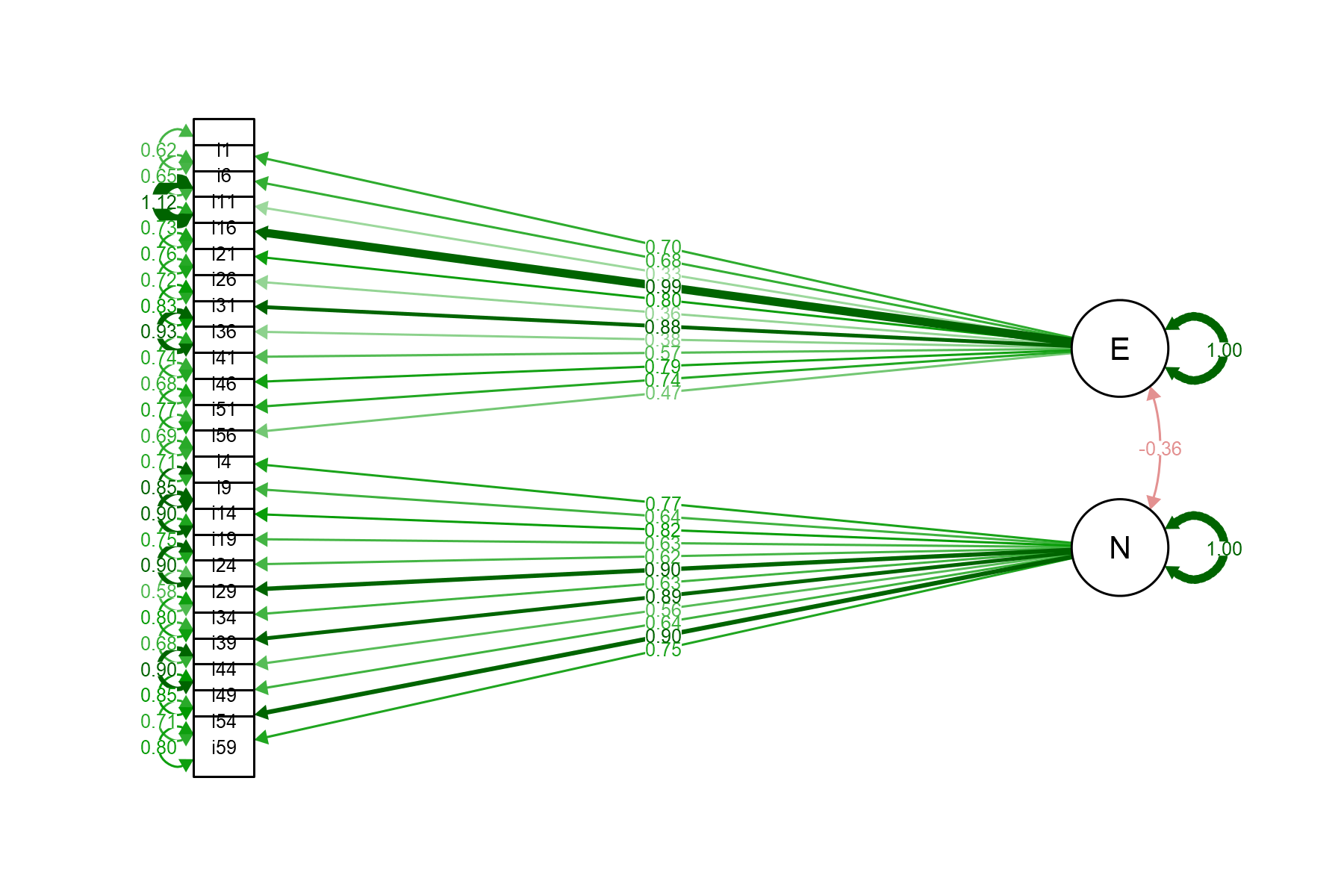
BFI2 dataset.
To predict the factor scores of individual respondents, we may use the predict() method on the fitted model. This returns a matrix of 2 columns (2 factor scores) for each of the 1,733 respondents. We have printed only the estimated factor scores for the first three respondents below.
FS <- predict(fit_EN)
head(FS, n = 3)
E N
[1,] 0.5944385 0.2344023
[2,] 0.6298318 -0.6943782
[3,] -1.4920334 1.6955088The first respondent had a level for extraversion 0.59 SD above average, and negative emotionality 0.23 SD above average, while the second respondent was above average in their level of extraversion and below average in negative emotionality. Finally, the third respondent seems to be well below average in extraversion and well above average in negative emotionality.
More complex latent variable models may be fitted with the lavaan package. The hierarchical or higher-order CFA allows for extra layers of latent variables. Such a hierarchical model was assumed in Hřebı́čková et al. (2020) and Soto & John (2017) for the BFI-2 instrument.
Hierarchical and more complex structures in lavaan. As before, we reduced the BFI2 dataset to items loading on the Extraversion and Negative Emotionality domains. We will now include information about facets hypothesized by the authors: The Extraversion domain is broken down to Sociability (scb) with items 1, 16, 31, and 46 loading onto it, Assertiveness (asr) with items 6, 21, 36, and 51, and Energy Level (enl) with items 11, 26, 41, and 56. Similarly, the Negative Emotionality domain is composed of Anxiety (anx) with items 4, 19, 34, and 49, Depression (dep) with items 9, 24, 39, and 54, and Emotional Volatility (emt) with items 14, 29, 44, and 59 loading onto it. In the lavaan package, the hierarchical structure is defined in model_EN_hier and fitted with the cfa() function as follows:
model_EN_hier <- 'Escb =~ i1 + i16 + i31 + i46
                  Easr =~ i6 + i21 + i36 + i51
                  Eenl =~ i11 + i26 + i41 + i56
                  Nanx =~ i4 + i19 + i34 + i49
                  Ndep =~ i9 + i24 + i39 + i54
                  Nemt =~ i14 + i29 + i44 + i59
                  E =~ Escb + Easr + Eenl
                  N =~ Nanx + Ndep + Nemt'
fit_EN_hier <- cfa(model = model_EN_hier, data = BFI2)
As before, summary of the model may be printed, model fit indices may be examined, and the estimated parameters and factor scores may be extracted and further inspected (see Supplementary R code). We plotted below the hierarchical CFA path diagram (Figure 3.6).
semPlot::semPaths(fit_EN_hier, what = "est", rotation = 4)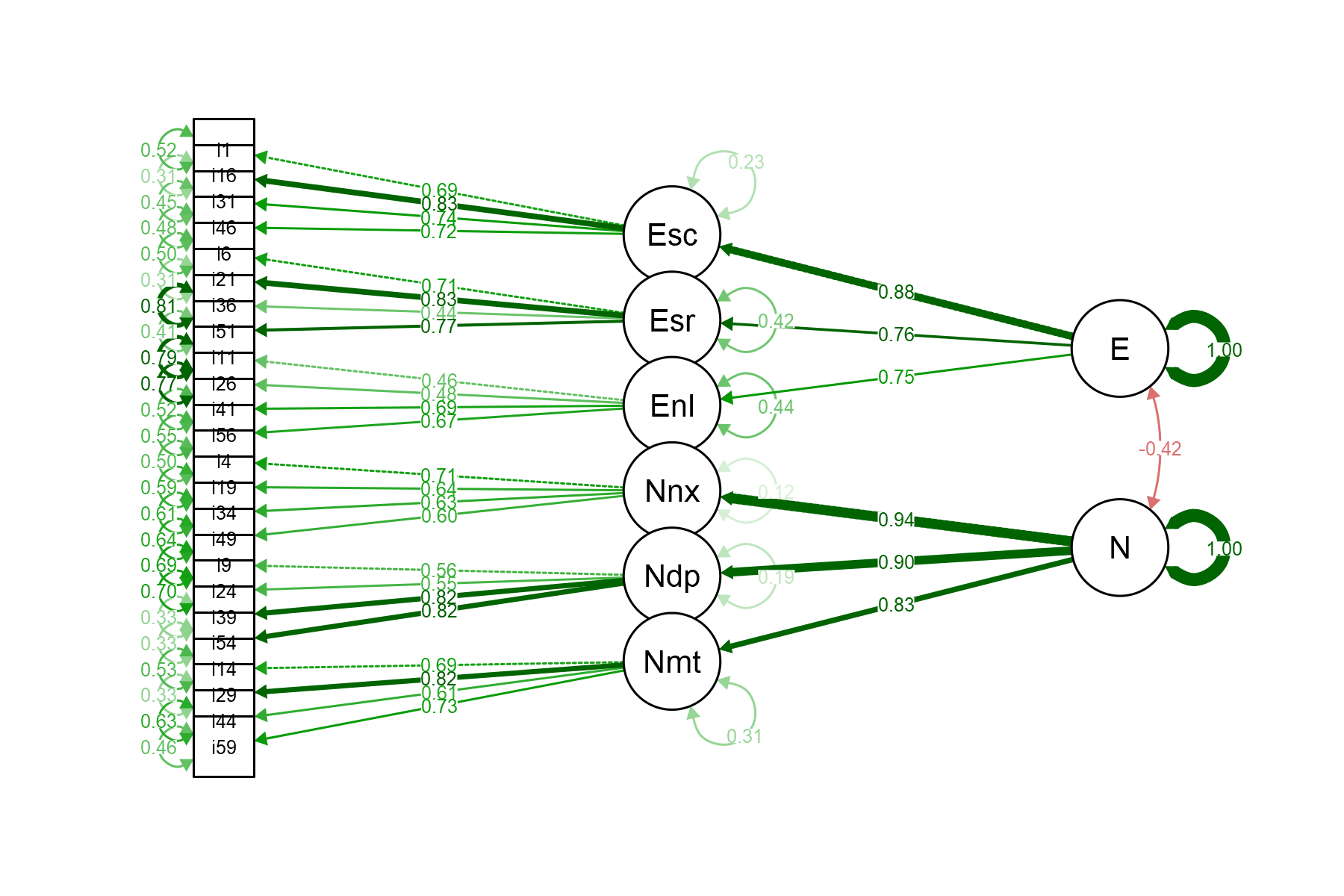
BFI2 dataset.
We can again use the predict() method to obtain estimated factor scores. We received 8 factor scores this time: 6 for the first level factors and 2 for the second level factors.
FSh <- predict(fit_EN_hier)
head(FSh, n = 3)
Escb Easr Eenl Nanx Ndep Nemt
[1,] 0.4400661 0.660283 0.5546291 -0.1260882 -0.1289223 0.8746602
[2,] 0.7308285 0.498353 0.3823355 -0.5643156 -0.7702824 -0.5637748
[3,] -1.5153368 -1.403458 -0.5332582 1.7516189 1.3824942 1.4776062
E N
[1,] 0.5130709 0.00408604
[2,] 0.6024881 -0.68316429
[3,] -1.2671214 1.66710924As before, the first respondent had an overall level for both the extraversion and the negative emotionality of above average, while the second respondent was above average in their level of extraversion and below average in negative emotionality. Finally, the third respondent seems to be well below average in extraversion and well above average in negative emotionality. The first level factor scores provide a more detailed picture. For example, with the third respondent, the low level of extraversion was especially due to low levels of sociability and assertiveness, while the high level of negative emotionality was especially due to high levels of anxiety.
In the lavaan package, the fitMeasures() function may be used to extract the model fit statistics. We printed only four: The BIC Equation 2.31, the CFI Equation 3.15, the TLI Equation 3.16, and the RMSEA Equation 3.14.
fitMeasures(fit_EN, c("cfi", "tli", "rmsea", "bic")) cfi tli rmsea bic
0.778 0.756 0.092 114975.452 fitMeasures(fit_EN_hier, c("cfi", "tli", "rmsea", "bic")) cfi tli rmsea bic
0.880 0.865 0.069 113303.631 A slightly better model fit (lower BIC and RMSEA, higher CFI and TLI) may be observed for the hierarchical model.
Under the section Validity, the ShinyItemAnalysis application, the tabs Correlation structure and Factor analysis offer validity proofs based on internal correlation structure, i.e., the correlations between the test items.
Correlation structure. In the Correlation structure section, to inspect the inter-item correlations, the user may choose from a number of correlation coefficients depending upon item types, including Pearson, Spearman, or polychoric. A selected coefficient is used to display a heat map with correlations between individual items. The values of estimated correlations may be displayed, and both matrix of correlation coefficients as well as the correlation heat-map may also be downloaded.
Further, the correlation heat map can be reordered using one of the hierarchical clustering methods described in Section 3.3. With a number of clusters larger than 1, the rectangles representing clusters are drawn. In the case of using a hierarchical clustering method, the corresponding dendrogram is also displayed.
Factor analysis. In the Exploratory factor analysis tab of the Validity section, the optimal number of factors can be examined using the scree plot, the parallel analysis, and various information criteria. For a selected number of factors, the EFA is offered (see Figure 3.7).
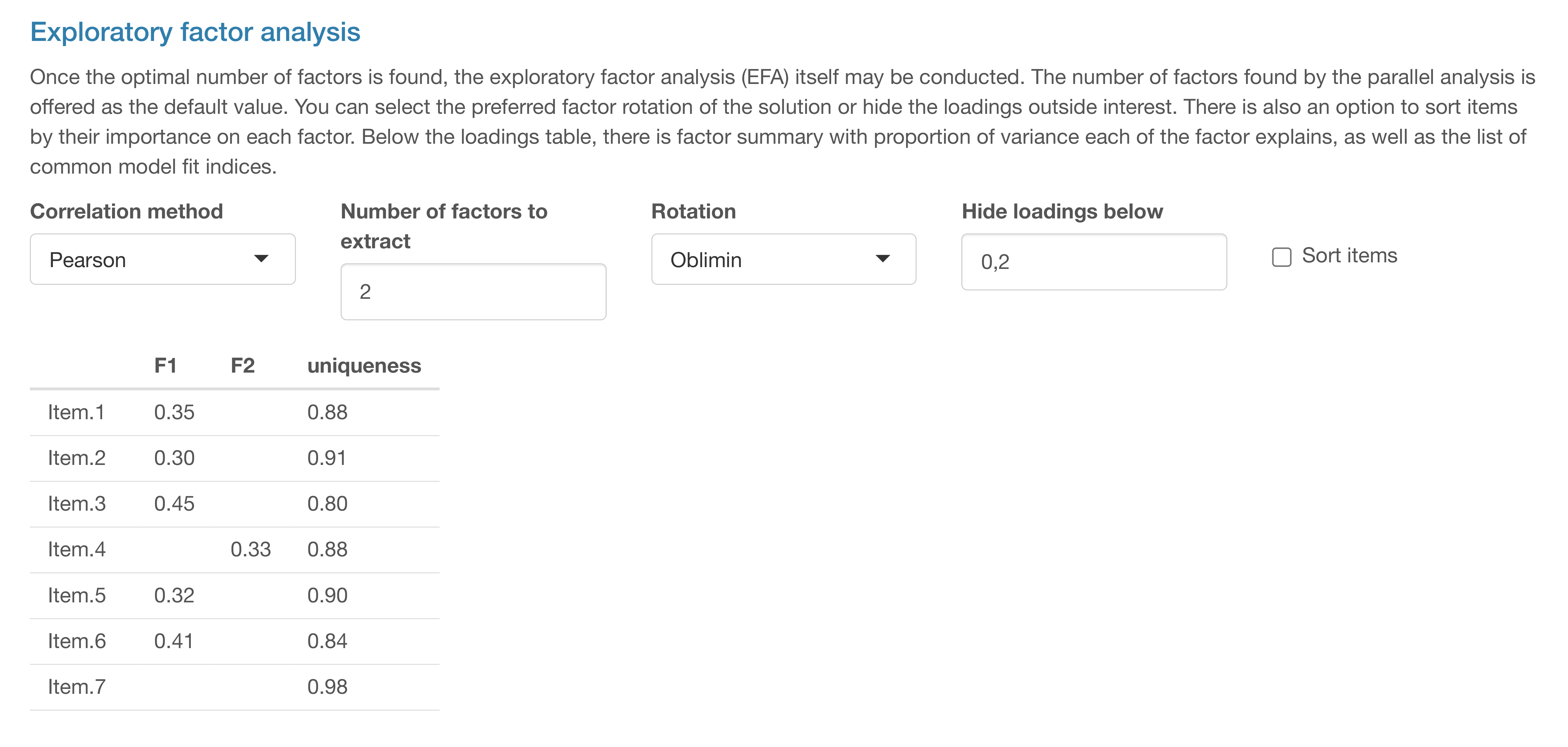
ShinyItemAnalysis.
In this chapter, we have discussed how to analyze the internal structure of a test in order to gain proofs of validity for a measurement instrument. We first discussed tetrachoric and polychoric correlation coefficients as an alternative to Pearson correlation coefficients in the case of binary or ordinal data. We then discussed how the correlation structure may be analyzed with cluster analysis. Finally, we took a latent variable modeling approach, and we discussed exploratory and confirmatory factor analysis.