# Probability mass function
x <- 0:20
pmf <- dbinom(x, size = 20, prob = 0.6)

barplot(pmf, names.arg = x, col = "steelblue",
        xlab = "Number of successes", ylab = "Probability",
        main = "Binomial(20, 0.6)")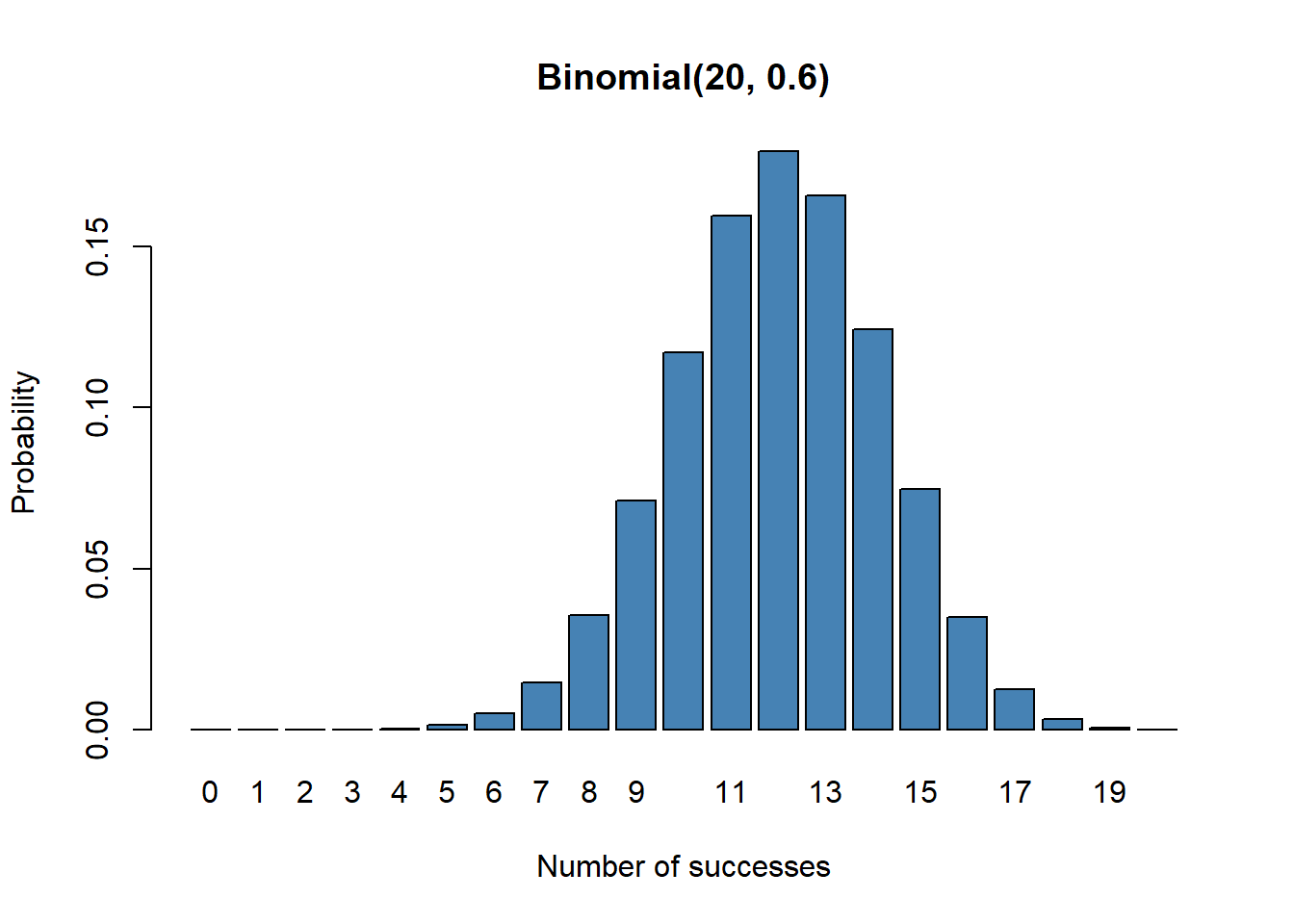
This appendix provides an overview of probability distributions commonly used in psychometric modeling.
The Bernoulli distribution describes a single trial with two possible outcomes: success (1) with probability \(\pi\) and failure (0) with probability \(1 - \pi\).
\[ P(Y = y) = \pi^y (1 - \pi)^{1-y}, \quad y \in \{0, 1\} \tag{C.1}\]
Properties:
This distribution is fundamental for modeling binary item responses.
The binomial distribution describes the number of successes in \(n\) independent Bernoulli trials, each with success probability \(\pi\). We write \(X \sim \text{Binomial}(n, \pi)\).
\[ P(X = x) = \binom{n}{x} \pi^x (1 - \pi)^{n-x}, \quad x \in \{0, 1, \ldots, n\} \tag{C.2}\]
Properties:
The binomial distribution is used when modeling total test scores under the assumption of equal item difficulties and local independence.
In R:
# Probability mass function
x <- 0:20
pmf <- dbinom(x, size = 20, prob = 0.6)
barplot(pmf, names.arg = x, col = "steelblue",
xlab = "Number of successes", ylab = "Probability",
main = "Binomial(20, 0.6)")# Mean and variance
n <- 20
pi <- 0.6
c(mean = n * pi, variance = n * pi * (1 - pi)) mean variance
12.0 4.8 The normal distribution (also called Gaussian distribution) is the most important continuous distribution. We write \(X \sim \mathcal{N}(\mu, \sigma^2)\) for a normal random variable with mean \(\mu\) and variance \(\sigma^2\).
The probability density function (PDF) is:
\[ f(x) = \frac{1}{\sigma\sqrt{2\pi}} \exp\left( -\frac{(x - \mu)^2}{2\sigma^2} \right) \tag{C.4}\]
Properties:
The standard normal distribution has \(\mu = 0\) and \(\sigma^2 = 1\), denoted \(Z \sim \mathcal{N}(0, 1)\).
In R:
# Density function
x <- seq(-4, 4, length.out = 200)
y <- dnorm(x, mean = 0, sd = 1)

plot(x, y, type = "l", lwd = 2, col = "steelblue",
     xlab = "x", ylab = "Density",
     main = "Standard Normal Distribution N(0, 1)")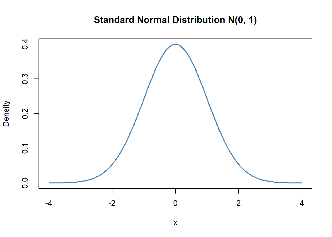
# Quantiles for confidence intervals
qnorm(c(0.025, 0.975))  # 95% CI boundaries
[1] -1.959964 1.959964qnorm(c(0.005, 0.995)) # 99% CI boundaries[1] -2.575829 2.575829The chi-square distribution with \(k\) degrees of freedom, denoted \(\chi^2_k\), arises as the distribution of the sum of \(k\) squared independent standard normal random variables.
\[ X = \sum_{i=1}^{k} Z_i^2, \quad Z_i \sim \mathcal{N}(0, 1) \tag{C.5}\]
Properties:
The chi-square distribution is used in likelihood ratio tests and goodness-of-fit tests.
In R:
x <- seq(0, 30, length.out = 200)
plot(x, dchisq(x, df = 2), type = "l", lwd = 2, col = "red",
     xlab = "x", ylab = "Density", ylim = c(0, 0.25),
     main = "Chi-square Distributions")
lines(x, dchisq(x, df = 5), lwd = 2, col = "blue")
lines(x, dchisq(x, df = 10), lwd = 2, col = "darkgreen")
legend("topright", legend = c("df=2", "df=5", "df=10"),
       col = c("red", "blue", "darkgreen"), lwd = 2)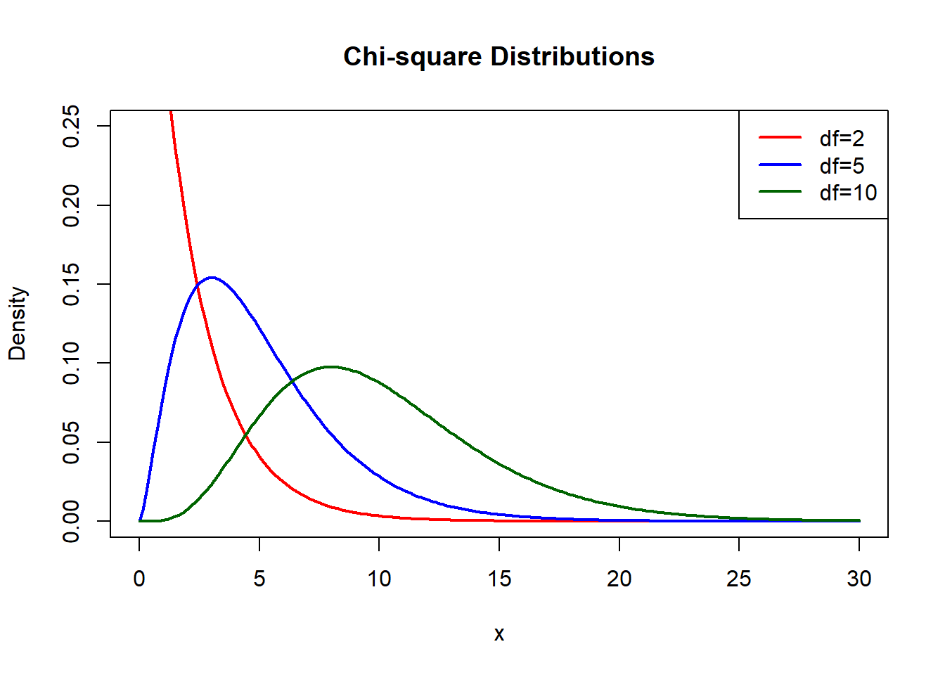
The Student’s t-distribution with \(\nu\) degrees of freedom, denoted \(t_\nu\), arises as the distribution of the ratio of a standard normal variable to the square root of a chi-square variable divided by its degrees of freedom.
\[ T = \frac{Z}{\sqrt{\chi^2_\nu / \nu}} \tag{C.6}\]
Properties:
The t-distribution is used for t-tests and confidence intervals when the population variance is unknown.
In R:
x <- seq(-4, 4, length.out = 200)
plot(x, dnorm(x), type = "l", lwd = 2, col = "black",
     xlab = "x", ylab = "Density",
     main = "t-Distributions vs Normal")
lines(x, dt(x, df = 3), lwd = 2, col = "red")
lines(x, dt(x, df = 10), lwd = 2, col = "blue")
legend("topright", legend = c("Normal", "t(df=3)", "t(df=10)"),
       col = c("black", "red", "blue"), lwd = 2)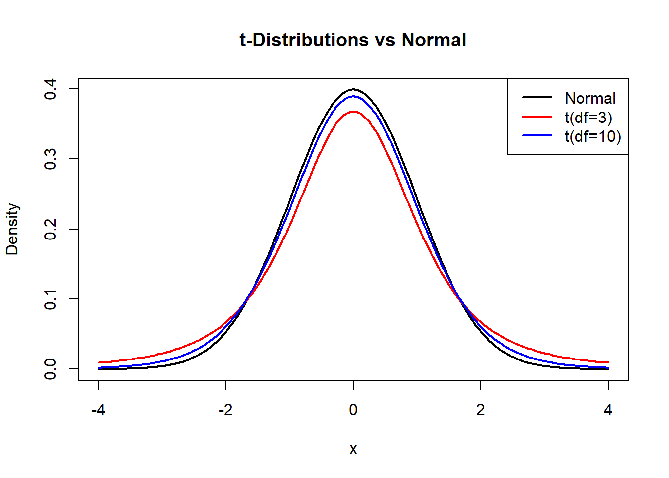
The F-distribution with degrees of freedom \(d_1\) and \(d_2\), denoted \(F_{d_1, d_2}\), arises as the distribution of the ratio of two independent chi-square variables, each divided by their degrees of freedom.
\[ F = \frac{\chi^2_{d_1} / d_1}{\chi^2_{d_2} / d_2} \tag{C.7}\]
Properties:
In R:
x <- seq(0, 5, length.out = 200)
plot(x, df(x, df1 = 5, df2 = 20), type = "l", lwd = 2, col = "steelblue",
     xlab = "x", ylab = "Density",
     main = "F(5, 20) Distribution")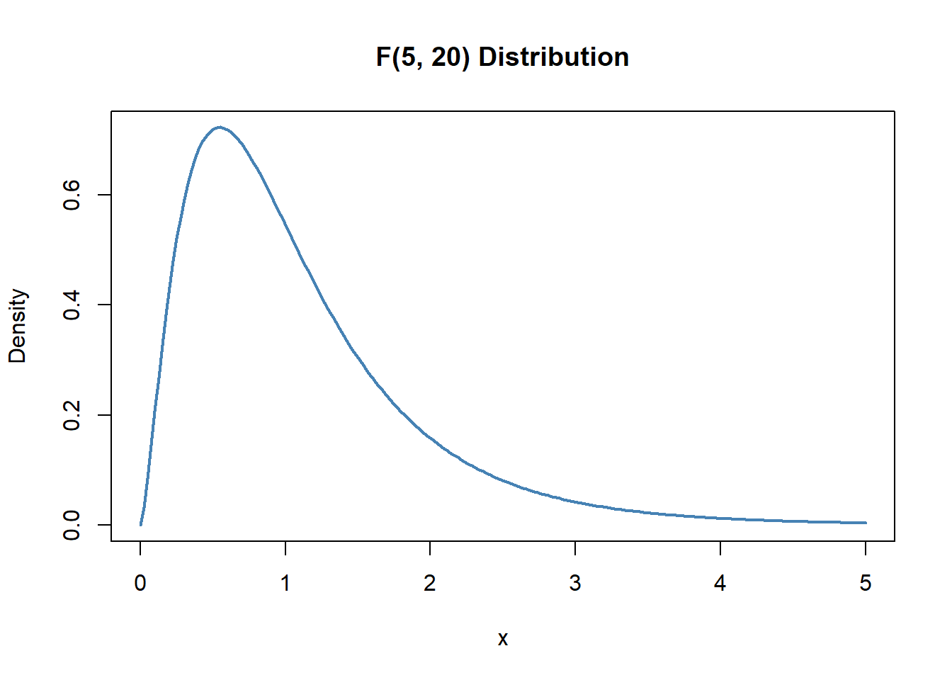
R provides four functions for each distribution:
| Prefix | Function | Description |
|---|---|---|
d |
dnorm(), dbinom(), etc. |
Density/probability mass function |
p |
pnorm(), pbinom(), etc. |
Cumulative distribution function |
q |
qnorm(), qbinom(), etc. |
Quantile function (inverse CDF) |
r |
rnorm(), rbinom(), etc. |
Random number generation |
Examples:
# Normal distribution
dnorm(0, mean = 0, sd = 1)  # Density at x = 0
[1] 0.3989423pnorm(1.96) # P(Z <= 1.96)[1] 0.9750021qnorm(0.975) # 97.5th percentile[1] 1.959964rnorm(5, mean = 0, sd = 1) # 5 random values[1] -0.7064627 -1.0130708 0.4829202 1.2553493 -0.6037007# Binomial distribution
dbinom(10, size = 20, prob = 0.5) # P(X = 10)[1] 0.1761971pbinom(10, size = 20, prob = 0.5) # P(X <= 10)[1] 0.5880985