Y <- c(34, 20, 34, 26, 27, 17, 22)
n <- 37
(p <- Y / n)
[1] 0.9189189 0.5405405 0.9189189 0.7027027 0.7297297 0.4594595 0.5945946One of the most fundamental considerations in the development and evaluation of educational, psychological, or health-related tests is their validity. Validity refers to the degree to which a test measures what it is intended to measure (Kelley, 1927). However, a single test can be used for multiple purposes; thus, to be more precise, validity describes the degree to which evidence and theory support the interpretations of the test scores for its proposed uses (AERA, APA, & NCME, (2014)).
Many classical statistical methods can be employed to gain empirical proofs of validity. In this chapter, we go over these essential statistical topics and discuss their use in the context of validity, while we leave some remaining topics for Chapter 3. We first provide an overview of different sources of validity evidence in Section 2.2. In Section 2.3, we discuss basic statistical methods involved in gathering empirical evidence of test validity: Inferences based on ratios, one-sample and two-sample \(t\) tests, ANOVA, correlation coefficients, and linear regression models. Further issues presented in Section 2.4 include parameter estimation methods, model fit, and the issue of range restriction. Finally, in Section 2.5, we discuss how tools for obtaining validity evidence based on external variables are implemented in the interactive ShinyItemAnalysis application.
To assess the degree to which evidence and theory support the interpretations of the test scores for its proposed use, the first step in test validation is the specification of the test’s proposed use and interpretation of the scores. An explicit statement regarding the proposed interpretation of test scores includes specifying the construct the test is intended to measure. In behavioral research, the construct refers to the concept, characteristic, status, or domain used to facilitate understanding of human behavior. Examples include self-esteem, depression, general cognitive ability, or mathematical achievement. More generally, constructs may also describe the quality of an applicant relative to a job position, grant application, or an institution.
To provide proofs of construct validity, test developers need to examine test content, its internal structure, and relationships to other, external variables. These are sometimes termed as types of validity (Cronbach & Meehl, 1955), aspects of validity, or sources of validity-supporting evidence (AERA, APA, & NCME, (2014)).
Proofs of content validity involve comparison of the content of the tests to the construct being tested. In educational testing, conceptual frameworks are built to describe the foundation stones of the domain being tested. Domain experts are invited to assure that all key ideas are present in the conceptual framework. For example, Michael et al. (2017) described the development of a conceptual framework for the core physiology concept of “cell-cell communication”. The framework consisted of hierarchically ordered ideas about cell-cell communication. The authors used ratings from domain experts to decide which of the ideas could be omitted, if the framework were to be shortened; they marked the ideas with less than 30% of the “essential” rating (5) as those that could possibly be skipped in testing the understanding of cell-cell communication.
Similarly, in a multi-stage process, McFarland et al. (2016) proposed and validated a conceptual framework for homeostasis with input from domain experts. Subsequently, when an educational test (the HCI) was developed and validated, content validity was established by assuring that test items covered all key ideas in the homeostasis conceptual framework (McFarland et al., 2017).
Relations to other, external variables may provide important sources of validity evidence. These aspects of validity are also sometimes termed criterion-related validity. We typically explore the strength of the relationship between test scores and a criterion measure. External variables may include scores from other tests hypothesized to measure the same, related, or different constructs, measures of criteria the test is expected to predict, group membership variables, or other respondent characteristics.
One of the goals is to demonstrate the test score is associated with variables that it should be associated with; this is usually termed convergent validity. For example, to demonstrate the convergent validity of the HCI, the scores on the test can be correlated with scores on other tests that are also designed to measure scientific knowledge. High correlations between the HCI test scores and the final grade in an undergraduate biology course, or more specifically in physiology, would be evidence of convergent validity.
Another aim is to demonstrate the test score is not associated with variables it should not be associated with, which is termed discriminant validity. For example, to provide proof of discriminant validity of an instrument measuring the level of narcissism, one may want to demonstrate that the scores from this instrument are not correlated too highly with scores from instruments designed to measure theoretically different concepts, such as intelligence.
When the criterion is measured at the same time as the test of interest, we talk about concurrent validity. For example, concurrent validity of an admission test may be examined by assessing the correlation of this test with another admission test.
When the criterion is measured subsequently, we talk about predictive validity. For example, the correlation with subsequent university success or university GPA may be used to demonstrate the predictive validity of admission scores. On the other hand, when the criterion has already been measured before taking the test, correlation of the test score with this criterion may be a proof of a retrodictive validity. An example of such proof might be the correlation of the leaving (matura) examination score in mathematics with previous grades in that subject.
We may also be interested in assessing incremental validity, i.e., providing proofs that the instrument of interest provides additional information. In the example of university admissions, we may evaluate if the admission test provides additional information about the applicant (e.g., in terms of their future university study success), other than an already existing test (such as the matura examination).
To assess criterion validity, the most common tool is the correlation coefficients between the total test score and the criterion variable. However, experimental evidence may be involved as well; for example, studies may be designed to investigate whether scores improve after therapy or whether scores on an achievement test differ between an instructed and an uninstructed group. Thus, other traditional statistical methods may be needed, such as \(t\) tests, ANOVA, or their nonparametric versions. Besides these methods, building a regression model allows accounting for a multiple number of covariates and their interactions; see Section 2.3.
Empirical evidence concerning the internal structure of the test is of high importance especially if the rationale for a test score interpretation depends on premises about the relationships among test items. For example, in personality research, the inventories are constructed to measure a multidimensional trait – in other words, to measure several personality characteristics at once. As a part of the validation process, the assumed internal structure needs to be confirmed empirically. In contrast, with educational research, it is usually claimed that the measured trait is unidimensional, and such a claim should also be empirically supported. The statistical methods involved are based on inter-item correlations, and may further involve multivariate methods such as cluster analysis, principal component analysis, or factor analysis, which we will more closely describe in Chapter 3.
We now turn our attention to statistical methods used in providing empirical evidence of test validity in real data examples. For more thorough introduction to statistical inference, the reader is referred to Dalgaard (2020).
Statistical inference based on ratios is useful in validation studies. For example, one proof of content validity (see Section 2.2.1) involves a statistical test of whether the ratio of experts who deem an item or an idea important is larger than what would be expected by pure chance.
The number of experts who deem an idea essential may be considered to be the realization of random variable \(Y\) following binomial distribution \(\textrm{Bi}(n, \pi)\), see Equation C.1 and Equation C.2. In this case the number of trials \(n\) is the number of experts giving their opinion and the probability of success in a single trial \(\pi\) is the true/population ratio of experts who deem the idea being essential.
In Section 1.6, we have shown that \(Y\) has an asymptotically normal distribution, \(Y \stackrel{\text{as.}}{\sim} \mathcal{N} (n \pi, n \pi(1 - \pi))\), see Figure C.1. Therefore, the standardized value
\[ Z = \frac{Y - n \pi}{\sqrt{n \pi(1 - \pi)}} \tag{2.1}\]
asymptotically follows a standard normal distribution, \(Z \stackrel{\text{as.}}{\sim} \mathcal{N} (0, 1)\). This fact can be readily used to determine whether the original number of experts is significantly higher than the predefined ratio \(\pi_0\) by simply checking whether \(Z\) is greater than a respective quantile of the standard normal distribution (1.96 in the case of a two-sided alternative, or 1.64 for a one-sided alternative).
If we consider the hypothesis \(\pi = 0.5\), that the idea is considered essential only by chance, the formula Equation 2.1 simplifies to
\[ Z = \frac{Y - \frac{n}{2}}{\frac{\sqrt{n}}{2}}. \tag{2.2}\]
This is very similar to the content validity ratio (CVR) proposed in Lawshe (1975) and widely cited in this context. Lawshe proposed CVR as
\[ \text{CVR} = \frac{Y - \frac{n}{2}}{\frac{n}{2}} = Z\frac{\sqrt{n}}{n}. \]
The resulting CVR does not asymptotically follow normal distribution and further calculations are needed to determine whether the original number of experts who deemed an item as important was beyond chance alone. For easy hypothesis testing, we prefer working with standardized counts as in Equation 2.1 and Equation 2.2 over the CVR.
Another option in statistical testing considers the squared value of Equation 2.1 which then asymptotically follows the \(\chi^2\) distribution Equation C.5 with one degree of freedom,
\[ Z^2 \stackrel{\text{as.}}{\sim} \chi^2_1. \tag{2.3}\]
Inferences based on ratios in R. As an example, let’s consider the validation of a cell-cell communication framework (Michael et al., 2017). We will consider only the seven key ideas and only the ratios of experts who considered the ideas as “essential”. Out of the 37 experts, 34 considered the first key idea as essential, and 20, 34, 26, 27, 17, and 22, respectively, considered the rest of the seven key ideas as essential, which corresponds to the percentages of 92%, 54%, 92%, 69%, 73%, 46%, and 59%.
Y <- c(34, 20, 34, 26, 27, 17, 22)
n <- 37
(p <- Y / n)[1] 0.9189189 0.5405405 0.9189189 0.7027027 0.7297297 0.4594595 0.5945946Considering the hypothesis that the number of experts who deemed the item as essential is above chance alone (\(\pi = 0.5\)), the standardized number of experts Equation 2.2 can be easily calculated in R and compared with the critical value – quantile of the standard normal distribution:
(Z <- (Y - n / 2) / (sqrt(n) / 2))[1] 5.096369 0.493197 5.096369 2.465985 2.794783 -0.493197 1.150793qnorm(1 - 0.05)[1] 1.644854For all but two of the key items (CC2 and CC6), the standardized number of experts is higher than the critical value of 1.65, suggesting that all but the two key items are considered essential by significantly more than half of the experts.
To demonstrate another option in statistical testing, we next consider the squared value \(Z^2\) Equation 2.3.
Z^2[1] 25.9729730 0.2432432 25.9729730 6.0810811 7.8108108 0.2432432 1.3243243This statistic is used by the base function prop.test() to calculate the confidence intervals for the true proportion \(\pi\).
One sided alternative is tested with an argument alternative = "greater". By default, the prop.test() function uses a continuity correction. Argument correct = FALSE can be used to enforce this correction not being used and the resulting \(\chi^2\) statistic is the same as calculated with Equation 2.3. Here we demonstrate the statistical test on the first idea, “A cell synthesizes a messenger molecule”, which was marked as essential by 34 out of 37 experts.
prop.test(x = 34, n = 37, alternative = "greater", correct = FALSE)
    1-sample proportions test without continuity correction

data:  34 out of 37, null probability 0.5
X-squared = 25.973, df = 1, p-value = 1.731e-07
alternative hypothesis: true p is greater than 0.5
95 percent confidence interval:
 0.813616 1.000000
sample estimates:
        p
0.9189189
For the case when an idea is marked as essential by 34 out of 37 experts, the ratio estimate is \(0.92\) with a confidence interval of \((0.81, 1.00)\) which does not cover \(0.50\). Beyond chance alone, the idea is considered essential by more than half of the experts (\(\chi^2\)-value = 25.97, p-value \(< 0.001\)).
Below, we provide calculations of p-values and confidence intervals for all the key ideas. We use the lapply() function to apply the prop.test() function on all items, which creates a list of 7 prop.test() outputs. We then use the sapply() function to extract the p-values and the confidence intervals into a data frame.
proptests <- lapply(Y, prop.test, n = n, alternative = "greater", correct = FALSE)
sapply(proptests, function(x) x$p.value) # p-values
[1] 1.731153e-07 3.109367e-01 1.731153e-07 6.831856e-03 2.596730e-03
[6] 6.890633e-01 1.249087e-01sapply(proptests, function(x) x$conf.int) # confidence intervals [,1] [,2] [,3] [,4] [,5] [,6] [,7]
[1,] 0.813616 0.4076601 0.813616 0.568782 0.5970975 0.3321039 0.4598256
[2,] 1.000000 1.0000000 1.000000 1.000000 1.0000000 1.0000000 1.0000000In summation, we see that ideas 1, 3, 4, and 5 were marked as essential by significantly more than half of the experts. Considering the fact that the respondents were evaluating the items on a scale of 1–5, we may test for ratios of interest other than \(\pi = 0.5\). In function prop.test(), the default value of argument p is \(0.5\), but it can be changed to other proportions of interest. For example, following the results, all seven main ideas are considered essential by a statistically higher proportion of experts than \(\pi = 0.3\), which was the ratio considered of interest in the original study.
Proofs of validity may involve comparison of a test score on two occasions, before and after treatment, such as learning or therapy. If the treatment is designed to change the subject’s levels of the measured construct, we would expect that the test score will significantly change. In other words, we expect that the pre-post differences will be significantly different from zero. The hypothesis about the changes in pairs of observations is tested with a paired \(t\) test. The paired \(t\) test is equivalent to the one sample \(t\) test applied on the differences, which we present in this section.
Formally, the one sample \(t\) test is designed to test whether the mean of a population deviates from the value specified by a null hypothesis. The test assumes an independent sample from a normally distributed variable. Independence is not testable, but should rather be deducted from the design of the experiment and data collection. The assumption of normality can typically be considered plausible with multiple-item measurements but can be inspected visually using a histogram or a QQ plot; see Figure 1.4 and Section 1.6. Under these assumptions, the \(t\) statistic
\[ t = \frac{\bar{X} - \mu}{\frac{s_{x}}{\sqrt{n}}} \tag{2.4}\]
follows a Student’s \(t\) distribution Equation C.6 with \(n - 1\) degrees of freedom (see Section C.2.3).
When considering the difference between two measurements (e.g., post-test score minus pre-test score), a one sample \(t\) test may be used to test the null hypothesis that the mean of the difference is zero. The two-sided alternative hypothesis states that the mean of the difference is not zero. Given the \(t\) distribution, the two-sided confidence interval for the mean \(\mu\) can be easily derived:
\[ \left(\bar{X} - t_{(n - 1), 1 -\alpha/2}\frac{s_{x}}{\sqrt{n}}, \bar{X} + t_{(n - 1), 1 - \alpha/2}\frac{s_{x}}{\sqrt{n}}\right); \tag{2.5}\]
see Exercise 2.2. Analogously, the one-sided confidence interval for the mean \(\mu\) can be derived (see Exercise 2.3), and the one-sided alternative of the post-test score being higher than the pre-test can be tested.
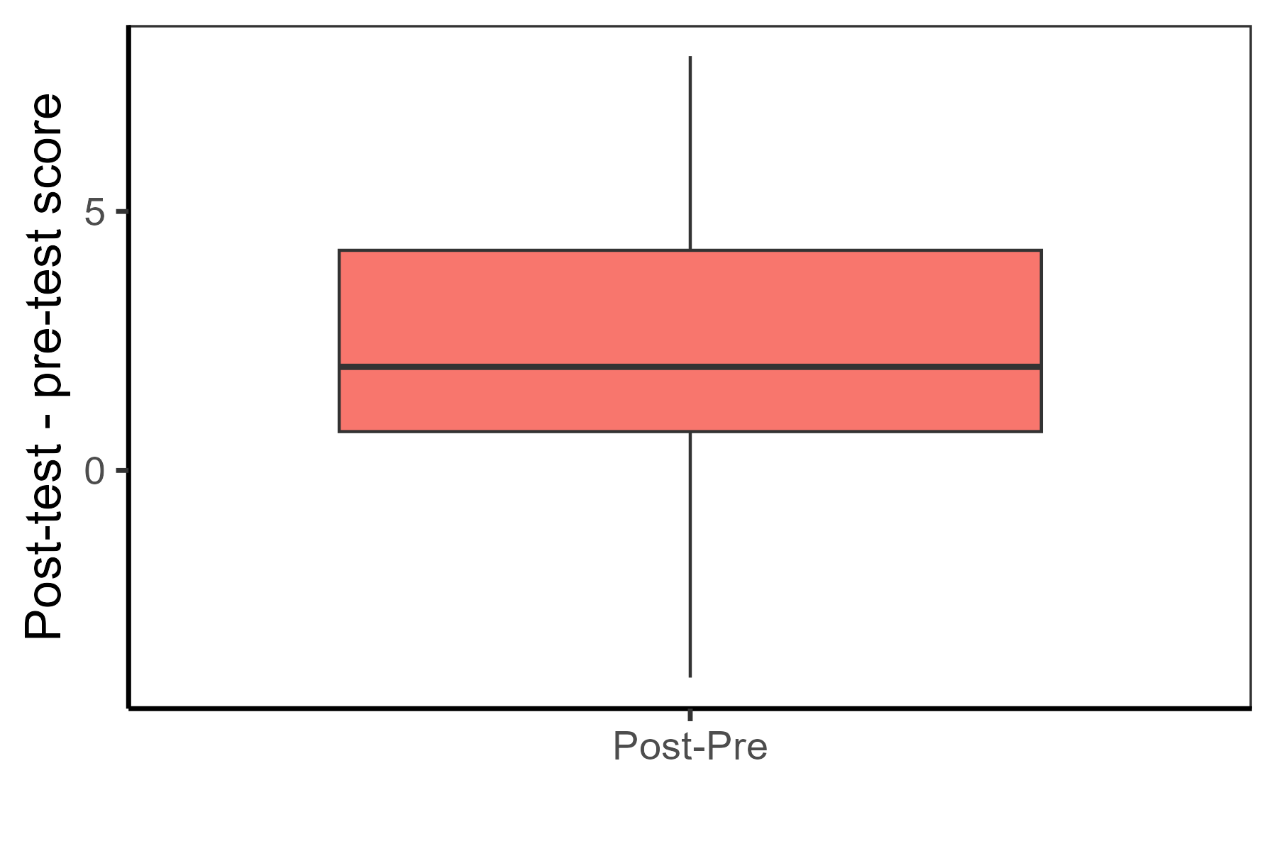
One sample and paired \(t\) test in R. In the following example we will examine how total scores of the HCI test changed after taking a course covering the concepts of homeostasis. We use the HCIprepost dataset of 16 students who took the HCI test before and after instruction on homeostasis received within a physiology course. We first display the differences between the pre-test and post-test scores using boxplots for pre-test and post-test, as well as for their difference. We load the data using the data() function, define the score vector combining the score.pre and score.post variables, and the group vector using the base rep() function for repeating levels "Pre" and "Post" 16 times each. We use the geom_boxplot() function from the ggplot2 package to construct the boxplot, and we use the earlier predefined theme theme_fig() while adding some extra layers, including the label of the \(y\) axis.
data(HCIprepost, package = "ShinyItemAnalysis")
ggplot(data.frame(
  score = c(HCIprepost$score.pre, HCIprepost$score.post),
  group = factor(rep(c("Pre", "Post"), each = 16),
                 levels = c("Pre", "Post"))),
  aes(x = group, y = score, fill = group)) +
  geom_boxplot() + ylab("Total score") + xlab("") +
  theme_fig() + theme(legend.position = "none")
Analogously, we display the boxplot for the pre-post differences:
ggplot(data.frame(
  score = HCIprepost$score.post - HCIprepost$score.pre,
  group = factor(rep(c("Post-Pre"), each = 16), levels = "Post-Pre")),
  aes(x = group, y = score, fill = group)) +
  geom_boxplot() +
  ylab("Post-test - pre-test score") + xlab("") +
  theme_fig() + theme(legend.position = "none")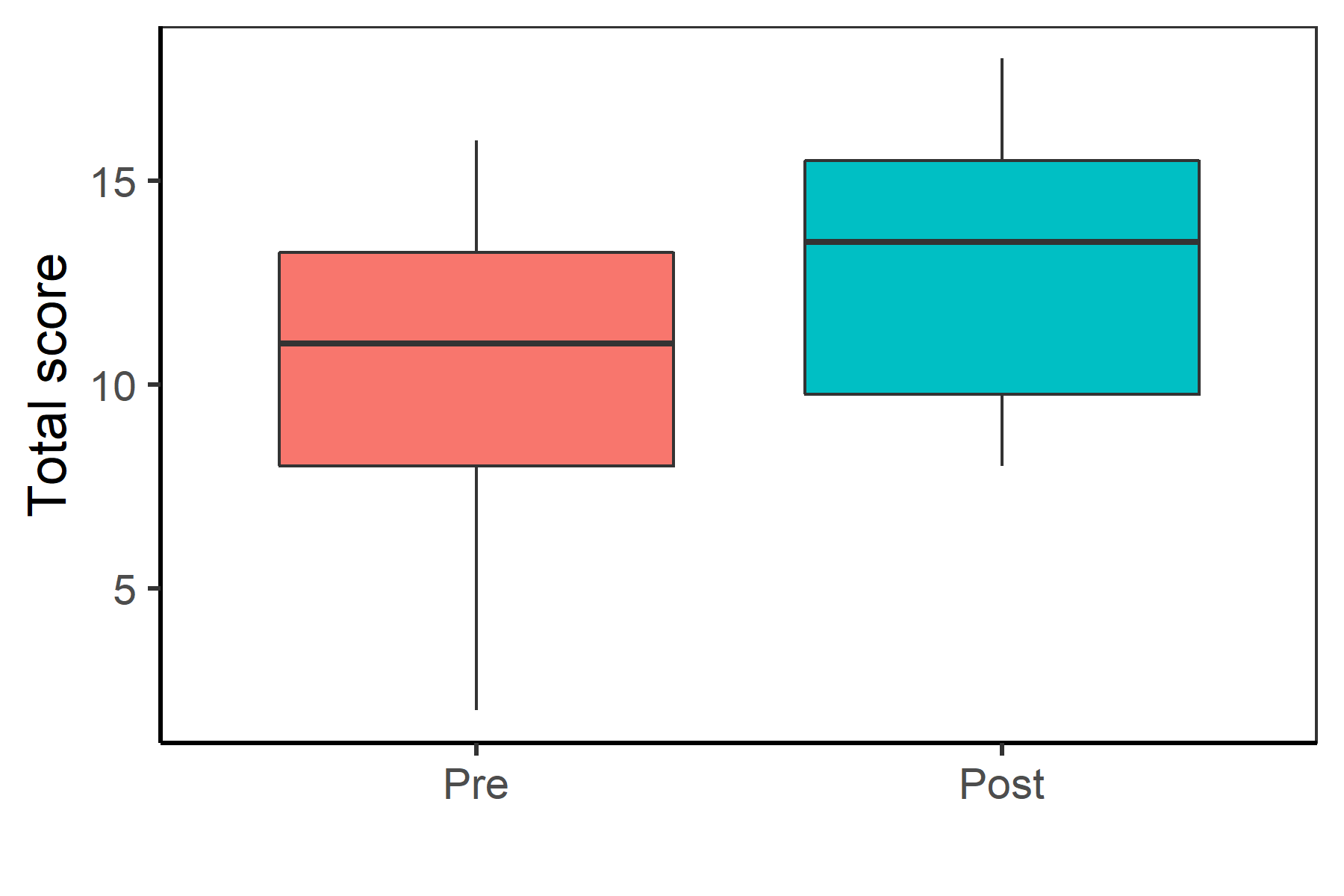
HCIprepost dataset.
There are apparent gains made after taking lessons on homeostasis (Figure 2.1): The post-test scores are somewhat higher than the pre-test score (Figure 2.1 (a)), and the difference of the pre-test and post-test score was thus above zero in most respondents (Figure 2.1 (b)).
To confirm the result with a one sample \(t\) test, the first option is to calculate the differences between the post- and pre-scores for all respondents. We first calculate the pre-post differences and the \(t\) statistics Equation 2.4. We then compute the corresponding confidence interval using the quantiles of the \(t\) distribution enumerated with the base qt() function. The p-value is calculated using the base pt() function.
data(HCIprepost, package = "ShinyItemAnalysis")
# differences between post-test and pre-test
(dif <- HCIprepost$score.post - HCIprepost$score.pre)
[1] 7 2 0 2 4 1 0 5 3 1 5 -2 4 8 1 -4(barX <- mean(dif)) # mean difference[1] 2.3125(sX <- sd(dif)) # standard deviation of difference[1] 3.156343n <- length(dif) # number of observations
(t <- barX / (sX / sqrt(n))) # t-value[1] 2.9306072 * pt(-abs(t), df = n - 1) # p-value[1] 0.01033258# confidence interval
barX - qt(1 -0.05 / 2, df = n - 1) * sX / sqrt(n)[1] 0.6306036barX + qt(1 - 0.05 / 2, df = n - 1) * sX / sqrt(n)[1] 3.994396The mean difference is \(2.31\) (SD = \(3.16\)). We reject the null hypothesis of there being no differences between the pre-test and post-test scores (\(t\) = \(2.93\), df = 15, p-value = \(0.01\)). The confidence interval of the mean difference between pre-test and post-test is \((0.63, 3.99)\) suggesting significantly nonzero gains after taking lessons on homeostasis.
Alternatively, one can apply the base t.test() function (which by default tests the null hypothesis that the mean is equal to 0) in the differences between pre-test and post-test scores. This yields exactly the same results:
t.test(dif, mu = 0)
    One Sample t-test

data:  dif
t = 2.9306, df = 15, p-value = 0.01033
alternative hypothesis: true mean is not equal to 0
95 percent confidence interval:
 0.6306036 3.9943964
sample estimates:
mean of x
   2.3125
Finally, one can see this as a comparison of two paired observations, which can also be analyzed with the t.test() function. Instead of applying the \(t\) test on the differences, the post- and pre-scores are employed with the argument paired = TRUE.
t.test(HCIprepost$score.post, HCIprepost$score.pre, paired = TRUE)
    Paired t-test

data:  HCIprepost$score.post and HCIprepost$score.pre
t = 2.9306, df = 15, p-value = 0.01033
alternative hypothesis: true mean difference is not equal to 0
95 percent confidence interval:
 0.6306036 3.9943964
sample estimates:
mean difference
         2.3125
This again gives the same result, the only difference being in wording of the alternative hypothesis, which now directly refers to the difference in means.
Proofs of criterion validity may also involve comparison of a test score for two groups. The two sample \(t\) test can be used to show that the measurement instrument is able to discriminate between groups as supported by the relevant theory. In this case, a group membership is considered a criterion variable. Examples include patients vs. healthy controls or knowledgeable vs. naive students (e.g., defined by their major or classes taken).
Formally, the two sample \(t\) test is designed to test the null hypothesis that the means of two populations are equal, \(H_0: \mu_x = \mu_y\). The \(t\) test assumes two independent samples \((X_1, \dots, X_{n_x})\) and \((Y_1, \dots, Y_{n_y})\) with normal distributions \(X_p \sim \mathcal{N} (\mu_x, \sigma^2_x)\) and \(Y_p \sim \mathcal{N} (\mu_y, \sigma^2_y)\). Two general cases of the \(t\) test are distinguished.
The first case assumes that the variances can be expected to be equal in the two groups, \(\sigma^2_x = \sigma^2_y = \sigma^2\), a property also termed as homoscedasticity. In this case, the following \(t\) statistic is considered:
\[ t = \frac{\bar{X} - \bar{Y}}{s_p \sqrt{\frac{1}{n_x} + \frac{1}{n_y}}}, \tag{2.6}\]
where \(n_x\) and \(n_y\) are the size of the first and the second sample, and \(s_p\) is a pooled standard deviation of the two samples, i.e.,
\[ s_p = \sqrt{\frac{(n_x - 1) s_x^2 + (n_y - 1) s_y^2}{n_x + n_y - 2}}. \]
It is known that under the null hypothesis \(H_0\), the \(t\) statistic Equation 2.6 follows the \(t\) distribution Equation C.6 with \((n_x + n_y - 2)\) degrees of freedom, which is used in hypothesis testing and derivation of the confidence interval for the mean difference between the two groups.
More generally, and for a case when the variances cannot be expected to be equal between the two groups (i.e., under a case of so-called heteroscedasticity), the Welch’s \(t\) test statistic (Welch, 1947) may be used with the test statistic
\[ t = \frac{\bar{X} - \bar{Y}}{\sqrt{\frac{s^2_x}{n_x} + \frac{s^2_y}{n_y}}} \tag{2.7}\]
which follows the \(t\) distribution with approximately \(f\) degrees of freedom, where
\[ f = \frac{\left(\frac{s^2_x}{n_x} + \frac{s^2_y}{n_y}\right)^2}{\frac{\left(\frac{s^2_x}{n_x}\right)^2}{n_x - 1} + \frac{\left(\frac{s^2_y}{n_y}\right)^2}{n_y - 1}}. \]
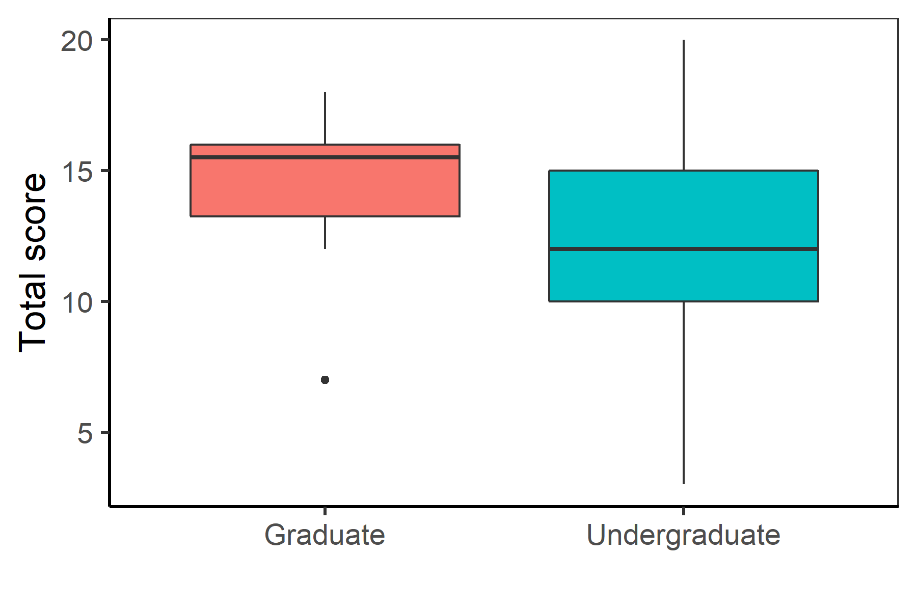
Two sample \(t\) test in R. As an example, let’s once again consider the HCI test. The dataset HCIgrads includes scores on the HCI test from 10 graduate students. To gain proofs of validity, we will compare the test scores of the graduate students with the test scores of the undergraduates in the HCI dataset. We expect, based upon theory and knowledge gained prior to the data collection, that the graduate students will receive higher scores than the undergraduates. We first calculate the total scores for both groups using the base rowSums() function.
data(HCIgrads, package = "ShinyItemAnalysis")
data(HCI, package = "ShinyItemAnalysis")
score_grads <- HCIgrads$total
score_undergrads <- HCI$total
It seems that graduate students achieved higher scores than undergraduates (Figure 2.2, see Supplementary R code).
The two sample \(t\) test is used to test for a difference in means between the undergraduate and the graduate students. As the default, the Welch’s \(t\) test Equation 2.7 is used, while the test assuming equal variances Equation 2.6 could be implemented specifying the var.equal = TRUE option (not shown here). The null hypothesis that there is no difference between the groups is tested against a one-sided alternative of a higher mean score in graduate students using the alternative = "greater" option:
t.test(score_grads, score_undergrads, alternative = "greater")
    Welch Two Sample t-test

data:  score_grads and score_undergrads
t = 2.1889, df = 9.3448, p-value = 0.02763
alternative hypothesis: true difference in means is greater than 0
95 percent confidence interval:
 0.3799544       Inf
sample estimates:
mean of x mean of y
 14.50000  12.21198
As expected, the mean total score for graduate students was higher (14.50) than for the undergraduates (12.21), with a one-sided confidence interval for the difference between the two groups of \((0.38, \infty)\), which does not cover 0. The difference between the two groups is thus significant (\(t\) = 2.19, df = 9.35, p-value = 0.03) and can be deemed to be evidence supporting the validity of the HCI. See Exercise 2.4 for other sources of evidence with the two sample \(t\) test.
While the \(t\) tests are generally considered to be robust with respect to violations of normality assumptions, outliers may negatively affect their power, especially with smaller sample sizes. Nonparametric alternatives to \(t\) tests typically use the same formulae while replacing the original values by their ranks within each group. This is the case with the Wilcoxon signed-rank test (Wilcoxon, 1945), a rank alternative to a one sample \(t\) test, or the Mann-Whitney U test (Mann & Whitney, 1947), which is a rank alternative to an independent samples \(t\) test.
Proofs of criterion validity may also involve a comparison of test scores across multiple groups. For example, a theory may imply that the level of knowledge differs for different school types given the different instruction involved, or that the level of anxiety differs in different diagnosis groups. An empirical test showing that test scores differ in these groups may then provide validity evidence using an external variable – in this case group membership.
Formally, the differences in the mean of a continuous variable (such as a test score) between more than two groups are tested with a statistical method termed analysis of variance, ANOVA (Fisher, 1934). If a single grouping variable is involved, i.e., dependence of the continuous variable on a single categorical variable is tested, the method is referred to as a one-way ANOVA.
The one-way ANOVA assumes \(K\) independent samples from normal distributions, specifically:
\[ \begin{split} & Y_{11}, Y_{12}, \dots, Y_{1n_1} \sim \mathcal{N}(\mu_1, \sigma_1^2),\\ & Y_{21}, Y_{22}, \dots, Y_{2n_2} \sim \mathcal{N}(\mu_2, \sigma_2^2),\\ & \dots\\ & Y_{K1}, Y_{K2}, \dots, Y_{Kn_K} \sim \mathcal{N}(\mu_K, \sigma_K^2). \end{split} \]
The null hypothesis tested by the one-way ANOVA is that the means are equal in all samples, that is \(H_0: \mu_1 = \dots = \mu_K = \mu\). It is customary to assume independence of observations and the homoscedasticity, that is equal variances among groups: \(\sigma^2_1 = \dots = \sigma^2_K = \sigma^2.\)
The other way of specifying the one-way ANOVA model is by the equation
\[ Y_{kp} = \mu + \beta_k + \epsilon_{kp} \]
where \(\mu\) is the overall mean, \(\beta_k\) is the group-specific mean, and \(\epsilon_{kp} \sim \mathcal{N}(0, \sigma^2)\) is a normally distributed random error of person \(p\) from group \(k\). The null hypothesis could then be reformulated as \(H_0: \beta_1 = \dots = \beta_K = 0\).
The test is an extension of the two sample \(t\) test Equation 2.6, for which the test statistic involved a difference in means for the two samples. In this case, we have \(K\) group means \(\bar{Y}_{1 \bullet}, \dots, \bar{Y}_{K \bullet}\), where \(\bar{Y}_{k \bullet} = \frac{1}{n_k} \sum_{p = 1}^{n_k} Y_{kp}\) for \(k = 1, \dots, K\). The differences between the groups are described by their variability from the overall mean \(\bar{Y}_{\bullet \bullet} = \frac{1}{K} \sum_{k = 1}^K \bar{Y}_{k \bullet}\).
The one-way ANOVA is based upon decomposition of the total squared deviations from the overall mean, denoted as the total sum of squares \(SS_T\) into two parts: One attributable to the difference between groups \(SS_G\) and one for the residual differences within groups \(SS_e\):
\[ \begin{split} SS_T =&\ \sum_{k = 1}^K\sum_{p = 1}^{n_k} \left(Y_{kp} - \bar{Y}_{\bullet \bullet}\right)^2, \\ SS_G =&\ \sum_{k = 1}^K\sum_{p = 1}^{n_k} \left(\bar{Y}_{k \bullet} - \bar{Y}_{\bullet \bullet}\right)^2, \\ SS_e =&\ \sum_{k = 1}^K\sum_{p = 1}^{n_k} \left(Y_{kp} - \bar{Y}_{k \bullet}\right)^2, \end{split} \tag{2.8}\]
where \(SS_T = SS_G + SS_e.\) The between-groups sum of squares \(SS_G\) has \(K - 1\) degrees of freedom, whereas the within-groups sum of squares \(SS_e\) has \(\sum_{k = 1}^{K} n_k - K\) degrees of freedom.
The mean squares are then defined as ratios of the sum of squares \(SS\) and their respective degrees of freedom:
\[ \begin{split} MS_G &= \frac{SS_G}{K - 1}, \\ MS_e &= \frac{SS_e}{\sum_{k=1}^{K} n_k - K}. \end{split} \tag{2.9}\]
Under the null hypothesis \(H_0\), they follow a \(\chi^2\) distribution Equation C.5 with respective degrees of freedom, more specifically, \(\chi^2_{K - 1}\) and \(\chi^2_{\sum_{k = 1}^{K} n_k - K}\) distribution. Thus, the ratio of the mean squares
\[ F = \frac{MS_G}{MS_e} \tag{2.10}\]
follows an \(F\) distribution Equation C.7 with respective degrees of freedom, more specifically the \(F_{K - 1, \sum_{k = 1}^{K} n_k - K}\) distribution. This \(F\) statistic is used for testing the null hypothesis: Large values of the \(F\) statistic suggest that there are significant differences between the group means, whereas small values close to 1 indicate that the between-group differences are negligible. When the value of the \(F\) statistic is larger than the respective critical value, the null hypothesis is rejected in favor of the alternative hypothesis of there being differences in group means.
If the null hypothesis is rejected, it may be of interest to subsequently decide in which pairs of groups the significant difference occurred. For this purpose, ANOVA may be complemented by the Tukey post-hoc comparison (Tukey, 1949). The Tukey test compares all possible pairs of means and implements a correction in order to account for multiple comparisons.
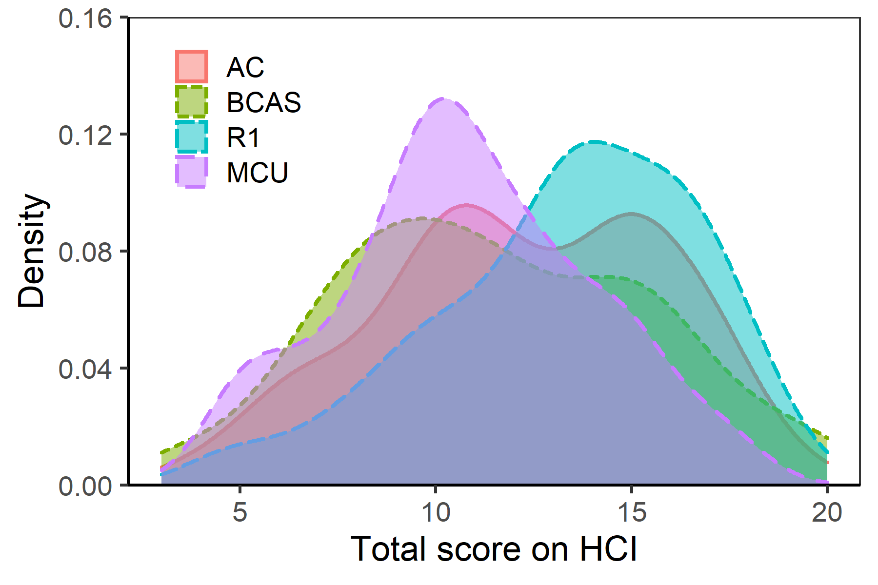
One-way ANOVA in R. As an example, let’s consider the scores from the HCI with respect to the institution type contained in the HCIdata. Students from four different institution types completed the HCI test. The expectation was that students from research universities R1 would score the highest.
Preliminary comparison regarding the group differences can be obtained using boxplots. A somewhat more detailed graphical description can be obtained with density plots using the geom_density() function within the ggplot() function of the ggplot2 package (see Supplementary R code). Higher scores seemed to be achieved by students from research universities than students from other institutions (Figure 2.3). The displayed densities suggest the highest scores for students from R1 institutions and a rather bimodal distribution for the students from associate’s colleges (AC), see Figure 2.3 (b).

To test the significance of the differences between the four groups, the ANOVA method can be implemented with the base aov() function.
data(HCIdata, package = "ShinyItemAnalysis")
anovaHCI <- aov(total ~ typeSCH, data = HCIdata)
summary(anovaHCI)
Df Sum Sq Mean Sq F value Pr(>F)
typeSCH 3 603 200.95 16.09 4.17e-10 ***
Residuals 665 8306 12.49
---
Signif. codes: 0 '***' 0.001 '**' 0.01 '*' 0.05 '.' 0.1 ' ' 1The summary() method provides the ANOVA table with rows for each effect (type of school effect and residual). The columns contain the degrees of freedom Df, sums of squares Sum Sq Equation 2.8, mean squares Equation 2.9, \(F\) statistics Equation 2.10, and respective p-value. The resulting statistic is far from its critical value and suggests the differences in means between groups are significant (F = 16.1, p-value \(< 0.001\)).
To subsequently decide in which pairs of institution types the significant difference occurred, we use the Tukey post-hoc comparison implemented within the TukeyHSD() function (HSD standing for the honest significant difference).
TukeyHSD(anovaHCI) Tukey multiple comparisons of means
95% family-wise confidence level
Fit: aov(formula = total ~ typeSCH, data = HCIdata)
$typeSCH
diff lwr upr p adj
BCAS-AC -0.6562896 -1.7002988 0.3877196 0.3685203
R1-AC 1.1536748 0.2456578 2.0616917 0.0061585
MCU-AC -1.4023939 -2.3982458 -0.4065420 0.0017518
R1-BCAS 1.8099644 0.7698916 2.8500371 0.0000514
MCU-BCAS -0.7461043 -1.8636810 0.3714723 0.3143014
MCU-R1 -2.5560687 -3.5477930 -1.5643444 0.0000000As expected, significant differences are confirmed between the research universities R1 and the other types of institutions, with R1 students receiving significantly higher scores. Moreover, significant differences are observed between associate’s colleges (AC) and master’s colleges and universities (MCU), with students from associate’s colleges performing better on average.
To establish criterion validity between the test and an external criterion (such as another, concurrent test), correlation coefficients may be used. For example, validity of the height inventory may be established by demonstrating a high correlation with actual height measured in centimeters.
Pearson’s \(r\) is the most popular correlation coefficient. Before describing its sample estimate, let’s start with the theoretical population value by extending the concepts described in Section 1.6.
The population covariance of two random variables \(X\) and \(Y\) with mean values \(\mu_X\) and \(\mu_Y\) is defined as:
\[ \sigma_{xy} = \text{Cov}(X, Y) = \text{E}\left(\left(X - \mu_X\right)\left(Y - \mu_Y\right)\right), \]
and the population correlation coefficient is defined as the ratio of population covariance \(\text{Cov}(X, Y)\) and the squared root of the product of their population variances \(\sigma^2_{X}\) and \(\sigma^2_{Y}\):
\[ \rho_{XY} = \frac{\text{Cov}(X, Y)}{\sigma_{X} \sigma_{Y}} = \frac{\text{E}\left(\left(X - \mu_X\right)\left(Y - \mu_Y\right)\right)}{\sigma_{X}\sigma_{Y}}. \tag{2.11}\]
Having real data, the population covariance and population correlation are estimated by their sample counterparts. Consider pairs of test scores \((X_{1}, Y_{1}), \dots, (X_{n}, Y_{n})\) from a sample of \(n\) respondents. The covariance can then be estimated by sample covariance \(s_{xy}\)
\[ s_{xy} = \frac{\sum_{p = 1}^n (X_{p} - \bar{X})(Y_{p} - \bar{Y})}{n - 1} \tag{2.12}\]
with \(\bar{X}\) and \(\bar{Y}\) being sample means. The sample Pearson correlation coefficient uses sample covariance \(s_{xy}\) Equation 2.12 and sample variances \(s^2_{x}\) and \(s^2_{y}\) Equation C.3:
\[ r_{xy} = \frac{s_{xy}}{s_{x} s_{y}} = \frac{\sum_{p = 1}^n (X_{p} - \bar{X})(Y_{p} - \bar{Y})}{\sqrt{\sum_{p = 1}^n (X_{p} - \bar{X})^2}\sqrt{\sum_{p = 1}^n (Y_{p} - \bar{Y})^2}}. \tag{2.13}\]
Values close to 1 represent a strong positive linear relationship, values close to \(-1\) represent a strong negative linear relationship, while values close to \(0\) represent a weak linear relationship. Values of \(1\) or \(-1\) are obtained when the observed values lie on a line.
When bivariate normal distribution of the variables can be assumed (this is the case when both \(X\) and \(Y\), as well as their sum \(X + Y\) are normally distributed, see Exercise 2.1), it may be shown that a certain function of \(r\), the so-called Fisher transformation, follows a Student’s \(t\) distribution Equation C.6 with \(n - 2\) degrees of freedom (Fisher, 1915):
\[ T = \frac{r}{\sqrt{1 - r^2}}\sqrt{n - 2} \sim t_{n - 2}. \tag{2.14}\]
This fact can be used to test the hypothesis that there is no correlation between the two variables \(X\) and \(Y\) and to derive confidence intervals of \(\rho\).
Besides establishing significance, an important aspect is the effect size, a sample-based value measuring the magnitude of a relationship or effect; in this case, the actual value of the sample correlation coefficient. Cohen (2013) suggests values for the sample correlation of \(0.10\), \(0.30\), and \(0.50\) which are indicative of a small, medium, and large correlation, respectively. However, these cutoffs are simply a rule-of-thumb, and therefore should be used with discretion. Also, since these recommendations are about correlation estimates, their uncertainty requires a confidence interval to be taken into account for interpretation.
Pearson correlation in R. As an example, let’s consider the HeightInventory dataset. We will use only data from those respondents with complete observations; other rows are discarded with the na.omit() function.
data("HeightInventory", package = "ShinyItemAnalysis")
HI <- na.omit(HeightInventory)
As evidence to support the validity of the HI, correlation between the test score (variable total) and the real height in centimeters (variable HeightCM) is explored here. We first take a look at the summary statistics for both variables.
summary(HI$total) Min. 1st Qu. Median Mean 3rd Qu. Max.
26.00 54.00 67.00 65.65 78.00 104.00 summary(HI$HeightCM) Min. 1st Qu. Median Mean 3rd Qu. Max.
145.0 165.0 171.0 172.2 179.0 207.0 The heights range from 145 to 207 centimeters with the mean height of 172.23 centimeters. The total scores from the HeightInventory dataset range from 26 to 104, with a mean score of 65.65.
To depict the relationship between the two variables, a scatter-plot can be constructed with the ggplot() and geom_point() functions from the ggplot2 package. We use the theme theme_fig() (see Section A.5.2) and the xlab() and ylab() functions to describe the axis of the plot.
ggplot(HI, aes(x = total, y = HeightCM)) +
  geom_point() + theme_fig() +
  xlab("HI score") + ylab("Height [cm]")
The higher the HI score is, the higher the actual height in centimeters (Figure 2.4), suggesting positive correlation between the two variables.
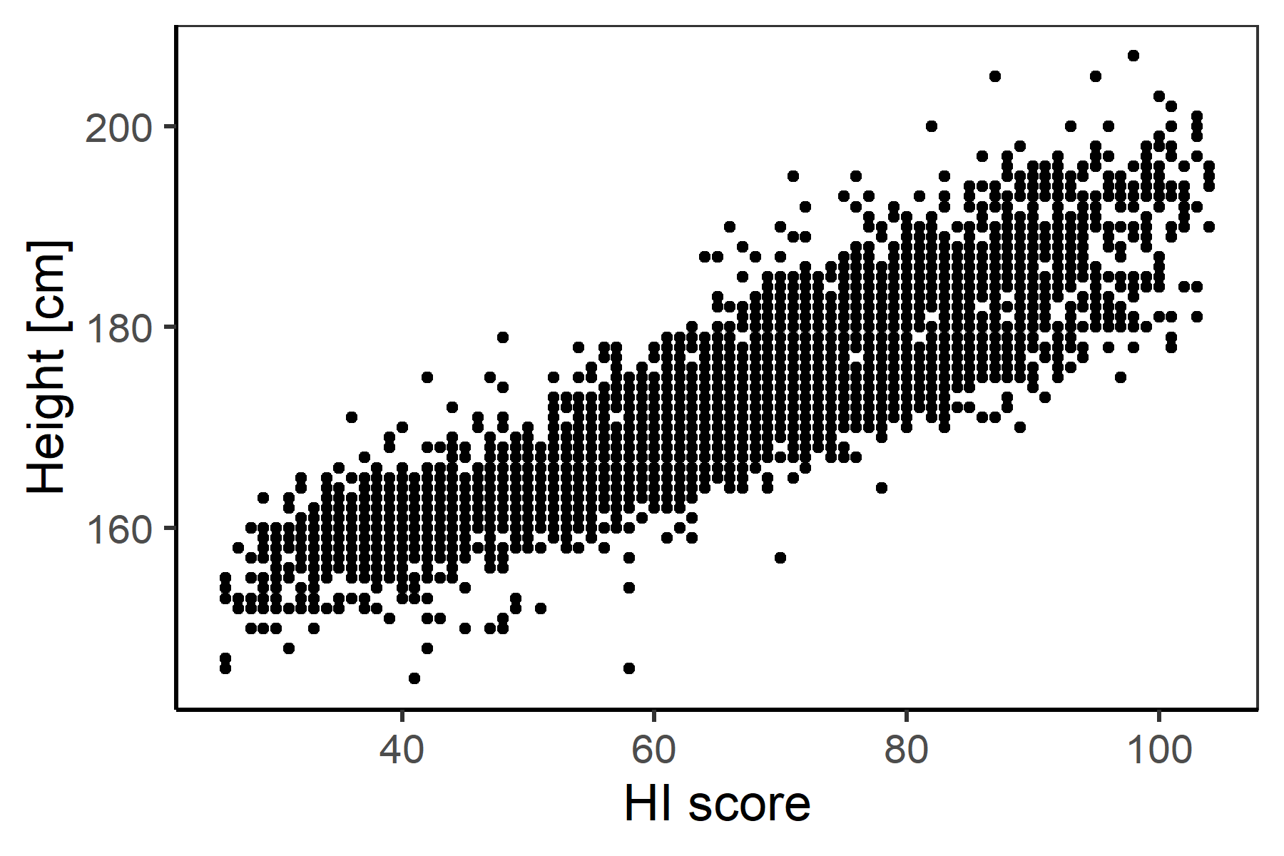
The base cor() function provides a point estimate of a sample correlation coefficient, while the cor.test() function also provides the \(t\) statistic Equation 2.14, degrees of freedom, p-value, and a \(95\%\) confidence interval, besides the point estimate, to test a nonzero correlation.
cor(HI$total, HI$HeightCM)[1] 0.8727557cor.test(HI$total, HI$HeightCM)
    Pearson's product-moment correlation

data:  HI$total and HI$HeightCM
t = 119.89, df = 4497, p-value < 2.2e-16
alternative hypothesis: true correlation is not equal to 0
95 percent confidence interval:
 0.8656099 0.8795461
sample estimates:
      cor
0.8727557
In this case, the resulting estimate of correlation is \(0.87\), with a confidence interval of \((0.87, 0.88)\), a large correlation, according to Cohen’s categorization. The confidence interval does not cover zero; thus the correlation is significantly nonzero (\(t\) = 120, df = 4497, p-value < 0.001).
In a case when one of the variables is binary (e.g., \(Y \in \left\{0, 1\right\}\) being a group membership, success/fail, or an indication of health status), the resulting estimate is referred to as a point-biserial correlation coefficient. The sample correlation coefficient Equation 2.13 can then be simplified to
\[ r = \frac{\bar{X}_1 - \bar{X}_0}{s_{n}}{\sqrt {\frac {n_{1} n_{0}}{n^{2}}}}, \tag{2.15}\]
with \(\bar{X}_0\) and \(\bar{X}_1\) being the sample means in the two groups defined by \(Y\), \(n_0\) and \(n_1\) their sample sizes, \(n = n_0 + n_1\) the overall sample size, and \(s_n = \sqrt{\frac{1}{n}\sum_{i = 1}^n (X_i - \bar{X})^2} = s_x \sqrt{\frac{n - 1}{n}}\) the standard deviation used when data are available for every population unit.
Point-biserial correlation in R. As an example, let’s consider the correlation between the test score and the gender of the respondent in the HeightInventory dataset. As we would expect the score was dependent on gender, the correlation between the two variables could be viewed as supporting evidence for test validity. We first multiply the factor variable gender by 1 to obtain a numerical variable.
HI$GenderM <- 1 * (HI$gender == "M")We then calculate the sample Pearson correlation using the cor.test() function. For a comparison, we also use the formula for a point-biserial correlation Equation 2.15 to show that it returns the same estimate.
cor.test(HI$total, HI$GenderM)
    Pearson's product-moment correlation

data:  HI$total and HI$GenderM
t = 29.093, df = 4497, p-value < 2.2e-16
alternative hypothesis: true correlation is not equal to 0
95 percent confidence interval:
 0.3731132 0.4223064
sample estimates:
      cor
0.3979959
barX0 <- mean(HI[HI$GenderM == 0, "total"])
barX1 <- mean(HI[HI$GenderM == 1, "total"])
n <- nrow(HI)
n0 <- sum(HI$GenderM == 0)
n1 <- sum(HI$GenderM == 1)
sn <- sd(HI$total) * sqrt((n - 1) / n)
(barX1 - barX0) / sn * sqrt(n0 * n1 / (n0 + n1)^2)[1] 0.3979959The point-biserial correlation between the HI test score and the gender variable is significantly nonzero, with an estimate of \(0.40\) and a \(95\%\) confidence interval of \((0.37, 0.42)\), suggesting that male respondents received a higher test score (\(t\) = 29.09, df = 4497, p-value < 0.001). According to the categorization by Cohen (2013) discussed above, the effect size of this correlation is medium to large.
The Pearson correlation coefficient is especially suitable for normally distributed data, and it is sensitive to outliers and deviations from a normal distribution of the variables. A more robust alternative is Spearman’s rank correlation coefficient (Spearman, 1904) which employs ranks to the original variables in the formula for Pearson’s correlation coefficient Equation 2.11. Another alternative is Kendall’s rank correlation coefficient (Kendall, 1938). In R, the cor() and cor.test() functions may again be used to calculate Spearman’s and Kendall’s correlation coefficients with the specified argument method = "spearman" or method = "kendall", respectively; see Supplementary R code for an example.
Correlation coefficients describe a mutual relationship between two variables. Regression models look at the data differently: They ask how well one of the variables, the dependent variable1, usually denoted by \(Y\), can be predicted by other variables, the independent variables2, which are usually denoted by \(X_1, X_2, \dots, X_m\).
There are two ways that regression models can be used to provide proofs of validity. The first way involves fitting a regression model with an assessment/test score as an independent variable. Proof of validity is obtained by demonstrating that the test score predicts some other variable of interest. As an example, to validate an admission test, one may be interested in proving that the test scores are able to predict subsequent student success. A regression model predicting height in centimeters based on the height inventory score, and possibly other covariates, may be used as a source of evidence of validity of the inventory.
The second way that regression models can be used to provide proofs of validity, which we will present, employs the test score as the dependent variable \(Y\) which is being modeled by either a single criterion or multiple criteria (predictors) such as respondent characteristics. The proofs of validity then involve demonstrating the differences in mean scores according to respondent characteristics, similar to the case for \(t\) tests and ANOVA, but allowing for multiple characteristics and for different types (continuous, ordinal, categorical), as well as their combinations.
In the case of a single continuous independent variable, the simple regression model assumes that the dependent variable \(Y_p\) is given by
\[ Y_p = \beta_0 + \beta_1 X_p + \epsilon_p, \tag{2.16}\]
where \(\beta_0\) is the intercept, \(\beta_1\) is the slope of the regression line, \(X_p\) is the dependent variable, and \(\epsilon_p \sim \mathcal{N}(0, \sigma^2)\) is a normally distributed error term, independent of \(X\), and with an unknown variance \(\sigma^2\). The assumption of normal distribution is important in order to make inferences.
The goal of a simple linear regression is to estimate the coefficients \(\beta_0\) and \(\beta_1\), in other words, to fit a straight line in the form \(y = \hat{\beta}_0 + \hat{\beta}_1 x\), which would best describe the points on the scatter-plot, such as those earlier depicted in Figure 2.4. The usual way of estimating this line is by using the method of least squares which involves minimizing the squares of the sum of the vertical deviations about the line, the errors, which are called residuals
\[ e_p = Y_p - \hat{\beta}_0 - \hat{\beta}_1 X_p = Y_p - \hat{Y}_p, \tag{2.17}\]
where the \(\hat{Y}_p = \hat{\beta}_0 + \hat{\beta}_1 X_p\) are the fitted values lying on the line. It can be shown algebraically that the sum of the squared deviations \(\sum_{p = 1}^n e_p^2\) are minimized for
\[ \hat{\beta}_1 = \frac{s_{xy}}{s^2_{x}} = r_{xy}\frac{s_{y}}{s_{x}} = \frac{\sum_{p = 1}^n (X_p - \bar{X})(Y_p - \bar{Y})}{\sum_{p = 1}^n (X_p - \bar{X})^2} \quad \textrm{and} \quad \hat{\beta}_0 = \bar{Y} - \hat{\beta}_1 \bar{X}. \tag{2.18}\]
Note that if \(X_p\) and \(Y_p\) have the same variability \(s_{x} = s_{y}\) (this can be achieved by standardizing the original measurements to Z-scores), then the slope \(\hat{\beta}_1\) is simply the sample Pearson correlation coefficient Equation 2.13.
Also note that the fitted value \(\hat{Y}_p\) is
\[ \hat{Y}_p = \hat{\beta}_0 + \hat{\beta}_1 X_p = (\bar{Y} - \hat{\beta}_1 \bar{X}) + \hat{\beta}_1 X_p = \bar{Y} + \hat{\beta}_1 (X_p - \bar{X}); \tag{2.19}\]
thus, the fitted regression line crosses through the mean point \([\bar{X}, \bar{Y}]\).
To measure the goodness of fit, i.e., the closeness of the points to the line, ANOVA is performed: The total variance of dependent variable, \(SS_T\), is split into the part explained by the regression, \(SS_R\), and a residual part, \(SS_E\):
\[ SS_T = \sum_{p = 1}^{n} (Y_p - \bar{Y})^2 = \sum_{p = 1}^{n} (\hat{Y}_p - \bar{Y})^2 + \sum_{p = 1}^{n} (Y_p - \hat{Y}_p)^2 = SS_R + SS_E. \tag{2.20}\]
The goodness of fit is then measured by a so-called coefficient of determination \(R^2\), the proportion of \(SS_R\) and \(SS_T\):
\[ R^2 = \frac{\sum_{p = 1}^n (\hat{Y}_p - \bar{Y})^2}{\sum_{p = 1}^{n} (Y_p - \bar{Y})^2} = \frac{SS_R}{SS_T}. \tag{2.21}\]
High values of \(R^2\) close to 1 mean close alignment to the linear regression curve. \(R^2\) is equal to the squared correlation between observed values \(Y_p\) and fitted values \(\hat{Y}_p\) and is thus easily generalized in cases of multiple covariates.
To test significance of the effect, an \(F\) statistic analogous to Equation 2.10 can be used
\[ F = \frac{MS_R}{MS_T} = \frac{SS_R / 1}{SS_T / (n - 2)} \sim F_{1, n - 2} \tag{2.22}\]
which has an \(F\) distribution with 1 and \(n - 2\) degrees of freedom.
To test whether \(Y_p\) linearly depends on \(X_p\) is equivalent to testing whether \(\beta_1 = 0\). To do so, we need to take a closer look at the distribution of the least-squares estimate \(\hat{\beta}_1\). This distribution can be derived from the model and Equation 2.19: Consider fixed pairs \((X_1, Y_1), \dots, (X_n, Y_n)\). Then \(\hat{\beta}_1\) has a mean of the true value \(\beta_1\) and a standard deviation depending on \(\sigma^2\), or more precisely \(\hat{\beta}_1 \sim \mathcal{N}\left(\beta_1, \frac{\sigma^2}{\sum_{p = 1}^{n} (X_p - \bar{X})^2}\right)\). With \(\sigma^2\) an unknown and being estimated, we end up with the test statistic following the \(t\) distribution Equation C.6 with \(n - 2\) degrees of freedom:
\[ T = \frac{\hat{\beta}_1}{\frac{S}{\sqrt{\sum_{p = 1}^{n} (X_p - \bar{X})^2}}} \sim t_{n - 2}, \tag{2.23}\]
where \(S\) is the squared root of the residual variance \(S^2 = \frac{\sum_{p = 1}^n (\hat{Y}_p - \bar{Y})^2}{n - 2}\). Notably, the \(T\) statistic Equation 2.23 is equivalent to Equation 2.14 which brings us back to the relationship between the slope parameter in the simple linear regression model and the Pearson correlation coefficient.
The assumptions of linear regression are the independence of variables, the linear relationship, normality, and constant variance (homoscedasticity) of the residuals. The assumption of independence is usually judged from the information about the source of the data. The normality of the residuals can be inspected visually by depicting the histogram or the QQ plot (see Section 1.6) for the residuals, while checking that the points lie approximately on a line. The assumption of linearity can be inspected by plotting the residuals against the fitted values and checking that the points lie approximately on the horizontal line around the zero.
Simple linear regression in R. We will now demonstrate fitting the linear line for predicting the height in centimeters HeightCM based on the HI total score. We start with calculating “by hand” in R computing the intercept and slope directly from Equation 2.18
(b1 <- cov(HI$total, HI$HeightCM) / var(HI$total))[1] 0.5018912(b0 <- mean(HI$HeightCM) - b1 * mean(HI$total))[1] 139.2778For an HI score of 0, the HeightCM is predicted to be around 139.28; however, this is a rather hypothetical situation given the lowest value of 145 centimeters for the height and the lowest HI score of 26 points. With an increase of one point on the HI score, the actual height is approximately \(0.5\) centimeters higher.
To add a regression line given by these coefficients to Figure 2.4, together with a confidence band around the regression line, we extend the original code by adding the geom_smooth() function from the ggplot2 package with an argument method = "lm" specifying the linear model and an argument se = TRUE to display the confidence band (Figure 2.5).
ggplot(HI, aes(x = total, y = HeightCM)) + geom_point() +
  geom_smooth(method = "lm", se = TRUE) +
  xlab("HI score") + ylab("Height [cm]") + theme_fig()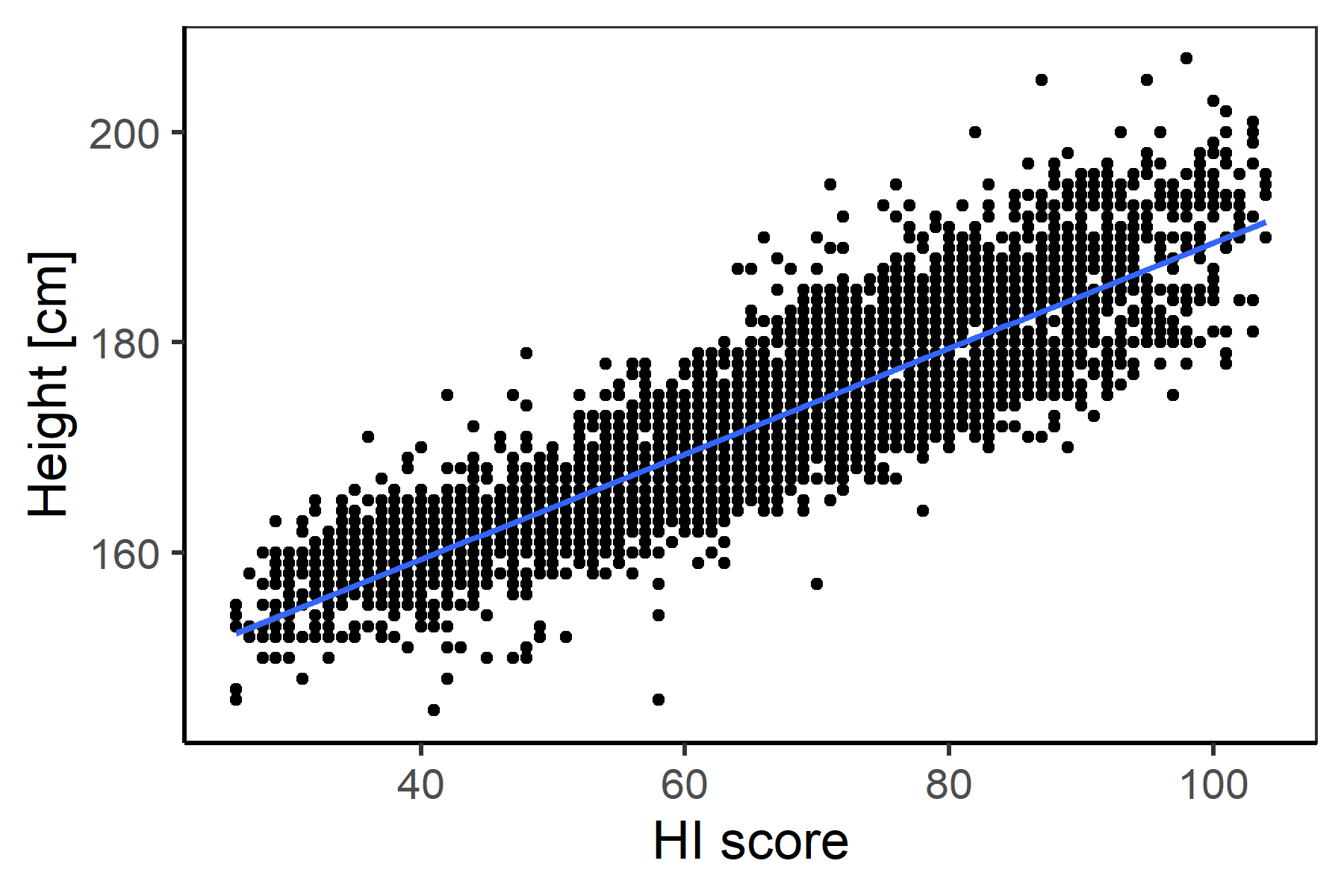
To fit the linear regression model, we use the base lm() function. The summary() method is applied to summarize the output:
lmHI <- lm(HeightCM ~ total, data = HI)
summary(lmHI)
Call:
lm(formula = HeightCM ~ total, data = HI)

Residuals:
     Min       1Q   Median       3Q      Max
-22.3875  -3.3989  -0.4026   3.1219  22.0576

Coefficients:
             Estimate Std. Error t value Pr(>|t|)
(Intercept) 1.393e+02  2.837e-01   490.9   <2e-16 ***
total       5.019e-01  4.186e-03   119.9   <2e-16 ***
---
Signif. codes:  0 '***' 0.001 '**' 0.01 '*' 0.05 '.' 0.1 ' ' 1

Residual standard error: 4.73 on 4497 degrees of freedom
Multiple R-squared:  0.7617,    Adjusted R-squared:  0.7616
F-statistic: 1.437e+04 on 1 and 4497 DF,  p-value: < 2.2e-16
The estimates of the intercept and the HI score effect are the same as before; this time, however, they are complemented with the standard errors and \(t\) statistic provided in Equation 2.23. The effect of the HI score (variable total) is about 139, significantly nonzero (\(t\) = 120, df = 4497, p-value < 0.001).
A summary of residuals \(e_p\) from Equation 2.17 displayed on the top of the output suggests no outliers and symmetrical distribution of residuals. Residuals for individual observations can also be obtained by using the output residuals of the lmHI object (see sample R code for alternative calculations).
lmHI$residuals 3 5 9 10 11 12
-6.37237785 -0.88939858 -3.88183381 8.65788122 -2.40263692 -1.45559029
14 15 16 17 18 19
-3.36859547 2.52549779 -6.94235195 -5.39507215 0.63140453 -3.92344003
20 21 22 23 24 25
7.09168951 -3.90074573 -6.93856956 -10.46315506 4.54819209 -3.90452811
26 27 28 29 30 31
1.12951334 2.13329573 18.04251852 -4.90831049 -4.84779236 0.55575686
32 34 35 36 37 38
1.10303666 -0.35724832 -3.37616023 7.08790712 2.65409884 -7.93856956
39 40 41 42 43 44
-1.93100480 -3.35346593 -4.90452811 -4.41398407 -0.90452811 5.66166360
46 48 49 50 51 52
-2.35724832 2.59736308 -4.87426904 1.62005738 -3.39507215 8.55197448
53 54 56 57 58 59
7.07655997 -9.38372500 2.15220764 -0.86292189 -3.91965764 4.15599003
60 61 62 63 64 65
-3.38750738 -1.88183381 10.03117137 -2.39507215 -0.91209288 -1.39128977
66 68 69 70 71 72
0.15977241 -2.40263692 -0.90074573 -3.35724832 -5.40641930 -0.86670427
73 74 75 76 77 78
2.07655997 -2.41020169 0.14464288 -4.84400997 -2.91587526 12.07655997
79 80 81 82 83 84
2.03495375 -2.40263692 -7.95369910 -5.94613433 -2.89696334 0.05764805
86 88 89 90 91 92
1.10303666 14.04630090 -2.84779236 -6.39507215 4.09168951 -0.88939858
93 94 95 96 97 98
-7.93856956 1.15977241 -1.86670427 -5.91587526 -0.87048666 -0.41776645
99 100 101 102 103 104
7.64275168 3.52549779 -4.91209288 -2.91209288 6.16733718 -5.44046075
105 106 107 108 109 110
-2.40641930 2.63518692 -5.95369910 -2.87805143 -0.39128977 -0.94613433
111 112 114 115 116 117
5.09547189 -4.86292189 6.09168951 -3.37994262 -1.90074573 -1.35346593
118 119 120 121 122 123
-1.88561619 1.14842526 8.60871023 -5.93478718 3.07277759 -4.40641930
124 125 126 127 128 129
-3.42533122 -2.89318096 -7.92722241 1.11816619 -4.38750738 7.05764805
130 131 132 133 134 135
7.06143044 -1.39885454 -1.87426904 -2.84779236 -3.94991671 3.08412474
136 138 139 140 142 143
-2.94613433 -2.90074573 -0.89318096 -0.37237785 1.62005738 3.60871023
144 145 146 147 149 150
-5.90452811 1.11816619 1.04630090 2.55953925 3.55953925 -5.42533122
152 153 155 156 157 158
-1.85535712 -9.43667837 1.13329573 -6.42911360 -3.91965764 0.56332163
159 160 161 162 163 166
2.63140453 1.09168951 -4.35724832 -2.92722241 0.60871023 -6.45559029
167 168 169 170 171 172
-0.35346593 1.65031645 9.66166360 2.57845116 6.60114546 5.06899520
173 175 176 177 178 179
-5.94235195 -0.37616023 5.55953925 4.08034236 -1.39885454 6.09168951
180 181 182 183 184 185
3.62005738 -2.37237785 -2.33833640 1.05764805 3.56332163 -7.92344003
186 187 188 189 190 191
-0.36103070 -5.42154884 -4.41776645 -4.42911360 -7.89696334 2.13707811
192 193 194 195 197 198
-2.42154884 0.12194857 6.57466878 5.65409884 3.59736308 2.55953925
199 200 201 202 203 204
-6.94613433 2.66166360 -4.91965764 -4.88183381 -2.41020169 1.13707811
205 206 207 208 209 210
5.63896930 -4.93856956 6.08790712 0.09168951 -4.93100480 -3.39885454
211 212 213 215 216 217
2.63518692 -3.39507215 8.03495375 -5.91587526 -3.92722241 5.14086049
218 219 221 222 223 224
-2.93478718 -8.46693744 -9.93478718 -4.41020169 -7.89318096 2.60114546
225 226 227 228 229 230
1.11438381 3.14464288 4.14464288 -6.39885454 1.58601593 3.16355479
231 232 233 234 235 236
-5.92722241 -4.46315506 0.13707811 -6.39128977 3.10303666 -5.92722241
237 238 239 240 241 242
-4.93100480 5.10681904 6.11060142 -4.41398407 6.58601593 5.55953925
243 244 245 246 247 248
6.05764805 2.05386567 -3.39885454 4.14842526 1.05764805 -5.91209288
249 250 251 253 255 256
-1.36103070 3.59736308 4.07655997 1.15977241 3.05386567 -3.88939858
257 258 259 260 261 262
-2.39128977 0.11438381 5.55953925 1.14464288 5.16355479 -1.86670427
263 264 265 267 268 269
-3.91965764 -5.92344003 2.14464288 -5.94235195 10.09925427 -3.88939858
270 271 272 273 274 275
6.07277759 3.12194857 -5.40641930 -2.91965764 -2.91965764 3.63896930
276 277 279 280 281 282
-0.90452811 4.04630090 -3.90074573 -0.33455401 -3.38750738 0.15220764
283 284 285 286 287 288
2.62383977 -6.87805143 -2.87805143 -1.41020169 7.57845116 0.66166360
289 290 291 292 293 294
-3.90831049 0.15599003 -1.91209288 5.14464288 -1.89318096 -1.88561619
296 297 298 299 300 302
-6.44424314 -4.42533122 -7.42911360 -4.41020169 -2.40263692 -6.93100480
303 304 305 306 308 309
0.54819209 -4.88561619 6.63896930 9.02738898 -2.91209288 -0.38750738
310 311 312 313 314 315
-3.90074573 0.12573096 0.14464288 -3.42154884 3.13329573 -2.39507215
316 317 318 319 320 321
1.65788122 0.14464288 5.58979831 -0.87426904 -2.41398407 -0.93856956
322 324 325 326 327 328
2.13329573 -4.92344003 -0.37237785 -6.39128977 -2.37994262 2.64653407
329 330 331 332 333 334
-5.90452811 5.08790712 -4.42154884 -3.40641930 -2.40641930 -5.40263692
335 336 337 338 339 340
1.58601593 -2.39885454 11.05008329 -1.42911360 3.04630090 0.12951334
341 342 343 344 345 346
-1.37616023 -7.89696334 -1.87048666 -1.88939858 0.65409884 0.11816619
347 348 349 350 351 353
-7.96126386 -3.94235195 -4.93478718 0.13329573 0.12951334 -0.43289599
354 355 356 357 358 359
-7.44046075 4.58979831 -4.38750738 -3.86292189 1.09168951 5.15599003
361 362 363 364 365 366
-0.90452811 0.12573096 -4.39885454 1.63896930 1.65031645 -1.36103070
367 368 369 370 371 372
2.55197448 -0.91587526 -5.91587526 -5.41776645 -2.91209288 -4.39885454
373 374 375 376 377 378
2.09547189 -9.45937267 -0.91209288 -2.38372500 0.63140453 -0.87805143
379 380 381 382 383 384
2.59736308 10.63140453 -2.43667837 -4.38750738 -1.94235195 -1.37994262
385 386 387 388 389 390
-2.84779236 -3.88939858 6.08034236 -7.92344003 -8.44424314 1.60114546
391 392 393 394 395 396
-3.41398407 2.13707811 -4.41776645 -0.87426904 -2.41020169 -5.96126386
397 398 399 400 401 402
-0.40263692 -3.38750738 -1.87805143 -0.87805143 -2.86670427 -2.87805143
403 404 405 406 407 408
-5.43289599 2.07655997 -3.90452811 -1.91965764 -2.90074573 -0.90831049
409 410 411 412 413 414
3.07277759 -0.37237785 2.13707811 -4.40263692 -1.88183381 0.05386567
415 416 417 418 419 420
-4.87426904 -0.88939858 -3.39885454 -2.41020169 -6.93100480 -0.37237785
421 422 423 424 425 426
0.63140453 -4.86670427 -7.38372500 -2.34968355 3.08412474 2.63518692
427 428 429 430 431 432
-4.34590116 -0.89318096 -2.41776645 -2.91587526 4.57466878 -4.38750738
433 434 435 436 437 438
-1.39507215 4.09925427 9.56710401 -1.94613433 -2.91209288 -6.95369910
439 440 441 442 443 444
-6.43289599 -0.37994262 2.15977241 -2.92722241 1.58223355 -3.96504625
445 446 447 448 449 450
3.57466878 -2.93100480 -4.85535712 2.04630090 1.54819209 -6.88561619
451 452 453 454 455 456
-0.95369910 1.14842526 3.58979831 -3.39885454 0.12573096 -0.89696334
457 458 459 462 463 464
2.05764805 3.64653407 2.62005738 -4.42911360 -0.92344003 -5.37237785
465 466 467 468 469 470
-5.41776645 -2.90452811 1.14086049 -3.36859547 5.09168951 -8.91965764
471 472 473 474 475 476
-6.93100480 2.58601593 -5.39128977 -1.89318096 -3.91965764 -0.40263692
477 478 479 480 481 482
-4.44802552 1.58979831 -5.91587526 -0.95369910 -3.39885454 -3.91209288
483 484 485 486 487 488
-9.95369910 2.14086049 -5.95748148 -8.44802552 1.59358070 -1.37616023
489 490 491 493 494 495
-1.88183381 -6.86670427 -5.89696334 -1.36859547 -4.95369910 -1.92722241
496 497 498 499 500 501
-4.42911360 -2.40641930 1.63896930 0.13707811 -4.42911360 3.14842526
502 505 506 508 509 510
-1.88183381 -1.41776645 4.57466878 -1.89696334 1.64275168 0.60114546
511 512 513 514 515 517
-1.38372500 -5.93100480 -3.91965764 -2.88183381 5.05008329 -11.94235195
518 519 520 521 522 523
-3.41398407 -0.39128977 -1.90074573 -8.41776645 3.63140453 -3.42154884
524 525 526 527 529 530
-6.91965764 2.15599003 -5.38750738 0.12951334 3.10681904 -2.88561619
531 532 533 534 535 536
2.65409884 -4.41398407 3.63140453 -3.89696334 -7.93100480 -2.42533122
537 538 539 540 541 542
5.05386567 -0.88939858 -0.84022759 -4.36481308 5.13329573 -5.37237785
543 545 546 547 548 549
-3.91587526 -0.37616023 5.57845116 -6.92722241 -6.96126386 -0.35346593
550 551 552 553 554 555
5.62762215 -1.89318096 5.56332163 1.55197448 -0.85913951 -1.93856956
556 557 558 559 560 561
-0.90831049 4.62762215 -3.36103070 -4.42911360 -2.90452811 -3.42533122
562 564 565 566 567 568
-3.40641930 -0.93478718 -1.41776645 -5.40263692 -3.41398407 -3.42911360
569 570 571 572 573 574
-0.91209288 -7.41776645 -0.88561619 -1.41398407 -1.37616023 -0.37616023
575 576 577 578 579 580
-1.88183381 -4.92722241 2.13329573 -1.86292189 -8.94613433 -4.40263692
581 582 583 584 585 586
-3.36103070 -1.91965764 1.07277759 -4.92722241 -1.91965764 -3.40641930
587 589 591 592 593 594
6.05386567 0.63140453 -0.39507215 5.14464288 7.11060142 1.11438381
595 596 597 599 600 601
5.62005738 0.11060142 -0.38372500 -4.40641930 -1.95369910 -0.89696334
603 604 605 606 607 608
-5.41398407 -0.40263692 -1.88561619 0.11816619 -1.88183381 -1.89318096
609 610 611 612 613 614
1.58223355 1.59736308 2.64653407 -6.44046075 1.09168951 -5.91587526
615 616 617 619 620 621
-2.43289599 -5.92722241 -9.42911360 -1.87805143 1.63140453 -3.40263692
622 623 624 625 626 627
-5.92722241 -4.92344003 0.66166360 1.65031645 0.61627500 8.10303666
628 629 630 631 632 633
3.16733718 1.65031645 -2.38372500 -3.41398407 -5.38750738 2.14464288
634 635 637 638 639 640
-1.43289599 -2.38372500 -3.96126386 4.14464288 4.13329573 -7.38372500
641 642 643 644 645 646
-5.92344003 -1.90452811 0.61627500 -8.93478718 -1.94991671 -3.89318096
647 648 649 650 651 652
-2.42533122 -0.42911360 -5.41776645 1.05386567 -4.89696334 -0.85913951
653 654 655 656 657 658
3.56710401 -3.39507215 6.11816619 0.10681904 3.06521282 -4.89318096
659 660 661 662 663 664
1.09925427 3.15599003 9.54062733 0.13329573 -8.42533122 4.64275168
665 666 667 668 669 670
-9.41776645 1.12951334 4.66544599 10.58979831 1.60492785 5.57088640
671 672 673 674 675 676
-1.45180791 -4.44802552 3.65409884 -2.40641930 6.11816619 -3.89696334
677 678 679 680 681 682
-1.36103070 -0.92722241 -0.87805143 0.63518692 -14.38750738 -0.87805143
683 684 685 686 687 688
7.06899520 -2.85913951 -1.85913951 -7.93100480 -1.45559029 2.13707811
689 690 691 692 694 695
-1.41776645 -5.93478718 -7.41776645 -1.37994262 2.54062733 -2.39507215
696 697 698 699 700 701
8.57088640 0.10681904 -4.93478718 -3.44802552 2.13707811 -2.37616023
702 703 704 705 706 707
6.53306256 7.57466878 -4.44802552 3.62762215 7.59736308 -6.90452811
708 709 710 711 712 713
-1.38750738 -3.90831049 -2.35346593 -3.87048666 2.15599003 -1.88939858
714 715 716 717 718 719
-4.87426904 2.13329573 -1.87805143 -3.89696334 -3.88561619 -2.89696334
720 721 722 723 724 725
-3.40641930 7.62383977 2.08790712 -4.36103070 -0.36103070 2.12573096
726 727 728 729 730 731
6.56332163 -1.85913951 -9.44802552 -2.89318096 4.14464288 -4.43289599
733 734 735 736 737 738
-8.43289599 3.59358070 4.12951334 -0.90452811 -0.86292189 -3.94613433
739 740 741 742 743 744
7.06521282 -1.39885454 3.64275168 -3.93100480 -0.34968355 15.09925427
745 746 747 748 749 750
-4.40263692 4.07277759 -0.42911360 -4.40641930 -5.44046075 -1.87805143
751 753 755 756 757 758
-0.86292189 -2.88183381 -5.44802552 -6.39507215 -9.38372500 -2.90452811
759 760 761 762 763 764
-2.90452811 8.03117137 -2.89696334 -1.41398407 -3.89696334 -0.34211878
765 766 767 768 769 771
0.10681904 -7.44424314 -7.46315506 0.63140453 -3.39885454 7.53684494
772 773 774 775 776 777
-0.86292189 5.15977241 -3.90831049 4.55197448 -3.90074573 3.04251852
778 779 780 781 782 783
-0.86292189 -2.90831049 -0.90452811 0.15220764 -4.39507215 5.08034236
784 785 787 790 791 792
2.63518692 -2.88939858 -6.95748148 -0.89696334 -0.87805143 -6.94235195
793 794 795 796 797 798
4.05386567 -3.40263692 -0.85913951 -5.93100480 8.06521282 -10.44424314
799 800 801 802 803 804
0.14464288 -0.38372500 -2.36481308 -0.93478718 -3.90831049 -4.42533122
805 806 807 808 809 810
-0.39128977 0.06899520 -5.35346593 -5.43289599 7.08412474 6.65031645
811 812 813 814 815 816
0.62762215 4.16733718 -0.39507215 -5.42533122 -0.87805143 -3.89696334
817 818 821 822 823 824
-1.90452811 -5.93478718 -7.44424314 -1.36103070 -3.41398407 0.66166360
825 826 828 829 830 831
-3.39885454 7.08790712 3.14086049 -2.42533122 -8.94613433 -5.39507215
832 833 834 835 836 837
-7.38372500 4.09547189 -2.91965764 -3.91587526 9.03495375 13.07277759
838 839 840 841 842 843
-1.39885454 -0.88939858 -0.42533122 -10.93478718 -0.83266282 -2.39507215
846 847 848 849 850 851
-4.40641930 2.15220764 18.53684494 8.58601593 2.58979831 -5.93856956
852 853 854 856 857 858
9.53306256 -2.90452811 -0.34211878 -1.85157474 10.56710401 5.07277759
859 860 861 864 865 866
-3.88939858 -0.87805143 -4.45559029 -10.45180791 -0.87426904 -0.37994262
867 868 869 870 871 872
0.60871023 6.06521282 1.10681904 -0.87805143 4.66166360 0.08790712
873 874 875 876 878 880
-0.38750738 -4.43289599 -3.41398407 -4.41776645 6.58223355 7.15599003
881 882 883 884 885 886
0.13329573 -2.89318096 -6.91209288 3.05764805 -1.35346593 1.12951334
887 888 889 890 891 892
0.09168951 1.11816619 -2.41776645 -6.41398407 2.10303666 -0.87805143
893 894 896 897 898 899
-1.47450221 5.08034236 -3.41398407 -0.39507215 -5.39507215 -1.34211878
900 901 902 903 904 905
-0.85157474 -5.40641930 -1.33077163 0.55953925 4.55953925 -7.45180791
906 907 908 909 910 911
0.08034236 -2.92344003 2.56710401 -0.90831049 3.57845116 -1.86670427
912 913 914 915 916 917
7.16355479 -0.40641930 -0.88183381 3.11060142 -0.36103070 -2.90452811
918 919 920 921 922 923
6.09168951 9.56710401 3.53684494 -4.40263692 -4.92722241 -1.88939858
924 925 926 927 928 929
3.12573096 -2.40263692 3.59358070 -2.44802552 -5.41776645 6.08412474
930 931 932 933 934 935
-4.41020169 -5.40263692 -3.88939858 5.11438381 -4.40263692 -5.45180791
936 937 938 939 940 942
-6.41398407 -5.46693744 -3.40263692 0.62762215 -1.90452811 1.63518692
944 945 946 947 948 949
-1.88183381 1.09925427 3.11816619 1.64275168 -10.87048666 4.66544599
950 951 952 953 954 955
4.56710401 0.61627500 1.55575686 1.13707811 13.65409884 -4.87805143
956 957 958 959 960 961
2.66166360 -5.41398407 0.15220764 1.58601593 2.59358070 -0.45559029
962 963 964 965 966 967
-1.36481308 -4.91209288 3.08412474 -1.92722241 1.15599003 2.13329573
968 969 971 972 973 974
-3.90831049 0.60871023 5.14842526 -3.92344003 0.11438381 0.57088640
975 976 977 978 979 980
2.57845116 0.13329573 -2.36859547 -8.43289599 3.12573096 3.06899520
981 982 983 984 985 986
-0.86292189 1.13707811 -7.92722241 -0.87426904 -3.37994262 -4.41398407
987 989 990 991 992 993
5.04630090 -0.87805143 -3.84022759 2.07277759 2.65031645 0.62383977
994 995 996 997 999 1000
-0.37237785 -0.36103070 11.55953925 10.61627500 -0.38750738 6.06899520
1001 1002 1003 1004 1005 1006
-4.90831049 -3.43289599 -4.35346593 0.06899520 5.05008329 14.64275168
1007 1008 1009 1010 1011 1012
-4.36481308 -7.40263692 -5.43289599 2.63518692 -2.88939858 -2.93478718
1013 1014 1015 1017 1018 1019
9.57088640 1.61627500 -1.40641930 16.58601593 -3.91587526 3.12573096
1020 1021 1022 1023 1024 1025
-2.90452811 -4.42911360 -4.86670427 -2.88183381 -0.85157474 5.54440971
1026 1027 1028 1029 1030 1031
5.56332163 -7.93856956 5.55953925 -5.43289599 3.58979831 -2.85913951
1033 1034 1035 1036 1037 1038
4.58601593 3.64275168 -2.88561619 -4.41776645 -4.92344003 -4.39128977
1039 1040 1041 1042 1043 1044
2.66544599 0.63896930 -5.91587526 -2.36481308 6.15599003 -1.90452811
1045 1046 1048 1049 1050 1051
-9.35724832 -6.41776645 -0.87048666 -1.89318096 1.09925427 -5.91587526
1052 1053 1054 1055 1056 1057
-1.84779236 -2.87426904 -5.91965764 6.11816619 -6.87426904 1.63518692
1058 1059 1060 1061 1062 1063
2.14842526 2.58223355 4.16355479 -3.89318096 -5.43289599 -5.90452811
1064 1065 1066 1067 1068 1069
7.09168951 -2.84022759 -3.40263692 3.54440971 0.52928018 0.10681904
1070 1071 1072 1073 1074 1075
-2.89318096 -4.85535712 -1.89696334 2.56332163 -0.89696334 -5.89696334
1076 1077 1078 1079 1080 1082
-1.37994262 0.08412474 1.12573096 -0.88939858 1.58223355 7.03117137
1083 1084 1085 1086 1087 1088
-4.44046075 -4.90074573 -5.43289599 -1.83266282 2.61249262 -7.40263692
1089 1090 1091 1092 1093 1094
1.57088640 -5.40263692 -2.87805143 -0.90074573 4.64275168 -3.95748148
1095 1096 1097 1098 1099 1100
-6.93856956 -3.41776645 0.62762215 4.08412474 -2.37994262 6.53306256
1101 1102 1103 1104 1105 1106
-7.42154884 -2.85913951 -0.36103070 -4.86670427 2.60492785 -6.45559029
1107 1108 1110 1111 1112 1113
-0.35724832 -3.34968355 6.63896930 1.14842526 -1.40641930 -4.91209288
1114 1115 1116 1117 1118 1119
11.05008329 3.55575686 6.56710401 3.09168951 -4.93478718 -1.37237785
1120 1121 1122 1123 1124 1125
-6.93856956 6.09925427 3.05764805 -1.43667837 5.17111956 5.63896930
1126 1127 1128 1129 1131 1132
-0.96126386 -4.40263692 5.15220764 4.58979831 5.10681904 6.09168951
1133 1134 1135 1136 1138 1139
-0.88561619 -0.36481308 2.11060142 6.56710401 3.05386567 -7.89696334
1140 1141 1142 1143 1144 1145
1.16733718 4.64275168 -0.91587526 10.14842526 -6.42533122 -3.94235195
1146 1147 1149 1150 1151 1152
-0.34211878 11.05764805 -1.41776645 -3.39885454 -1.39507215 -4.91965764
1153 1154 1155 1156 1157 1158
0.08412474 1.13329573 4.09168951 -4.92722241 -8.90452811 3.08034236
1159 1160 1161 1162 1163 1164
4.07277759 -0.87048666 7.58979831 1.61249262 3.57845116 -3.94991671
1165 1166 1167 1168 1169 1170
2.14086049 0.11438381 1.54819209 -8.45559029 9.07277759 0.64653407
1171 1172 1173 1174 1175 1176
-4.41020169 3.12573096 5.05386567 2.13707811 -5.42911360 -7.96126386
1177 1178 1179 1180 1183 1185
-4.40641930 3.05008329 9.08034236 1.16355479 -1.37616023 1.07277759
1186 1187 1188 1189 1190 1191
-1.91965764 1.60114546 0.15220764 -2.89696334 -0.88183381 -0.39507215
1192 1194 1195 1196 1197 1198
0.11060142 7.57845116 0.12573096 -3.90452811 -1.86292189 -7.36859547
1199 1200 1201 1202 1203 1204
-3.37237785 1.07277759 2.57088640 -14.42533122 1.14086049 9.05764805
1205 1206 1207 1208 1209 1210
1.63518692 2.07277759 -2.90831049 -0.38750738 -1.87048666 2.63140453
1212 1213 1214 1215 1216 1217
-3.45559029 -4.40641930 1.08790712 -11.94991671 0.64653407 -2.89318096
1218 1219 1220 1221 1222 1223
-4.38372500 -4.40263692 3.14842526 -4.45937267 -3.86670427 -1.38372500
1224 1225 1226 1227 1228 1229
-1.88939858 2.63518692 -1.37994262 -1.90831049 1.09547189 -2.90452811
1230 1231 1232 1233 1234 1235
-8.40263692 1.08790712 4.16733718 -11.96882863 -6.44802552 -5.84779236
1236 1237 1238 1239 1240 1241
-4.38372500 -3.87048666 1.63140453 6.62383977 -3.41398407 -4.39507215
1242 1243 1244 1245 1246 1247
-1.89318096 1.06143044 1.08034236 -7.42533122 -5.40641930 2.56710401
1248 1249 1250 1251 1252 1253
-2.90074573 4.58601593 -3.90074573 5.09168951 -3.90074573 -6.39885454
1254 1255 1256 1257 1258 1259
1.64275168 5.08034236 12.58979831 5.56710401 -3.90074573 3.57088640
1260 1261 1262 1263 1264 1265
-3.90074573 -0.89696334 2.61627500 4.59358070 1.63518692 -2.88561619
1266 1267 1268 1269 1270 1271
-3.43289599 5.65409884 -4.34968355 -4.41776645 -1.91587526 2.13707811
1272 1273 1274 1275 1276 1277
-0.40263692 -0.39128977 -1.35346593 -7.39507215 1.64275168 -2.91209288
1278 1279 1280 1281 1282 1283
-1.84779236 -4.40641930 -0.90831049 1.64653407 5.04630090 -2.39885454
1284 1285 1286 1287 1288 1289
-4.41020169 3.08790712 1.05764805 5.57845116 -5.35724832 -2.90074573
1290 1291 1292 1293 1294 1295
-2.92344003 9.02738898 -0.43289599 1.11060142 1.64275168 -3.88939858
1296 1297 1298 1299 1300 1301
-1.39885454 2.09547189 -1.35346593 -3.39128977 -2.88561619 -1.87426904
1302 1304 1305 1306 1307 1309
-5.92344003 1.11816619 -4.33455401 4.12194857 -6.85535712 -2.44046075
1310 1311 1312 1313 1314 1316
-1.89696334 -4.37994262 -2.43289599 -4.88939858 3.64653407 5.65031645
1317 1318 1320 1321 1323 1324
2.11438381 8.58979831 -3.39885454 -5.42154884 -4.44046075 0.66544599
1325 1326 1327 1329 1331 1332
-7.42154884 9.58223355 6.08034236 1.56710401 -0.90074573 -1.37616023
1333 1334 1335 1336 1337 1338
-1.41020169 1.08412474 2.07277759 -0.38372500 -5.92722241 -0.93478718
1339 1340 1341 1342 1343 1344
2.13707811 -5.41020169 2.04630090 6.08412474 2.63896930 3.16355479
1345 1346 1347 1348 1349 1350
-1.37994262 -4.94991671 -8.41776645 -1.91587526 -0.41020169 1.63518692
1351 1352 1353 1354 1355 1356
-6.43667837 11.05386567 2.09925427 -7.44046075 -4.88939858 1.03495375
1357 1358 1359 1361 1362 1363
4.60492785 -1.92722241 -1.90831049 -3.92722241 6.05386567 -1.90074573
1364 1365 1366 1367 1368 1369
1.15599003 -1.89318096 3.61249262 -6.94991671 -3.38750738 -1.86292189
1370 1371 1372 1373 1374 1375
-5.37616023 -5.88561619 -7.39128977 0.09168951 10.11438381 3.07655997
1376 1377 1378 1379 1380 1381
-1.39128977 -3.43289599 6.02738898 -2.40263692 6.03495375 -13.94613433
1382 1383 1384 1385 1386 1387
-9.91965764 -4.39128977 0.63896930 -5.39128977 4.57466878 2.65031645
1388 1389 1390 1391 1392 1393
-3.41776645 4.65409884 -4.88939858 0.11060142 5.55953925 -0.35346593
1394 1395 1396 1397 1398 1399
-5.90074573 -1.37994262 0.09547189 5.10303666 -0.34968355 4.14464288
1400 1401 1402 1403 1404 1406
5.03495375 4.06521282 -1.90074573 -1.86670427 -2.91209288 -2.36103070
1407 1408 1409 1410 1411 1412
-11.86292189 0.54440971 4.07655997 1.14842526 -6.88183381 -4.92344003
1413 1414 1415 1416 1417 1418
-0.88939858 2.57466878 -3.88561619 1.57466878 2.57466878 -3.39128977
1419 1420 1422 1423 1424 1425
1.09168951 -1.84779236 -2.88561619 -5.94613433 2.10303666 -6.41398407
1426 1427 1428 1429 1430 1431
9.05386567 -4.91965764 -1.35346593 -4.89318096 1.62005738 -3.87048666
1432 1433 1434 1435 1436 1437
2.60492785 -1.37616023 -2.88183381 -0.35724832 -5.89318096 -0.95369910
1438 1439 1440 1441 1442 1443
4.64653407 -2.41398407 22.05764805 8.54819209 -4.42154884 -2.40641930
1444 1445 1446 1447 1448 1449
0.64275168 9.57088640 4.03873614 -3.90831049 -0.42911360 3.11060142
1450 1451 1452 1453 1454 1455
2.11438381 0.04630090 1.13707811 4.55197448 2.08034236 -2.91209288
1457 1458 1459 1460 1461 1462
-0.88561619 -6.94991671 -3.42533122 -9.93856956 0.11438381 -6.93478718
1463 1464 1466 1467 1468 1469
-1.34968355 4.60492785 1.09168951 6.10681904 5.09547189 4.58223355
1470 1471 1472 1473 1474 1475
-5.90831049 6.03495375 -0.91965764 -1.90074573 6.60114546 -2.91209288
1476 1477 1478 1479 1480 1481
-7.91209288 5.11438381 -12.36859547 0.16733718 -4.92344003 -4.36481308
1482 1483 1484 1485 1486 1487
-1.91209288 2.08412474 -0.86292189 -22.38750738 1.63518692 5.15599003
1488 1489 1490 1491 1492 1493
2.61627500 3.65788122 -1.39885454 1.12951334 11.62005738 0.63518692
1495 1496 1497 1498 1499 1500
-3.87805143 5.16733718 -0.90452811 -3.39885454 1.12951334 0.67301075
1501 1502 1503 1504 1505 1506
-0.39885454 -4.39507215 -4.42911360 2.07655997 3.65788122 8.60871023
1507 1508 1510 1511 1512 1513
-5.91209288 -0.87426904 -2.39128977 -1.37994262 1.12194857 7.59736308
1514 1515 1516 1517 1518 1519
-3.91965764 0.12951334 -3.90074573 -1.90452811 -2.41398407 -4.44046075
1520 1521 1522 1523 1525 1526
2.63518692 0.12194857 2.65031645 0.14086049 0.58979831 7.55953925
1527 1528 1530 1531 1532 1533
-2.41020169 -1.85157474 1.09168951 2.63518692 -2.90074573 2.52928018
1534 1535 1536 1537 1538 1539
-2.41020169 -8.90452811 -4.36481308 -1.37994262 -1.87426904 6.09168951
1540 1542 1543 1544 1546 1547
2.14086049 1.60114546 -2.39507215 8.08034236 -2.40263692 -2.89696334
1548 1549 1550 1551 1552 1553
4.11060142 0.57088640 -6.36103070 -1.90831049 -4.93100480 -6.43289599
1554 1555 1556 1557 1558 1559
-5.92722241 -4.41020169 -2.84779236 -0.86670427 -3.90074573 -3.92722241
1560 1561 1562 1563 1564 1565
-12.87426904 -0.36481308 -7.93478718 -3.92344003 -0.91587526 -0.38372500
1566 1567 1568 1569 1570 1571
-1.84779236 5.58223355 4.08790712 -7.89318096 2.65031645 4.60114546
1572 1573 1574 1575 1576 1577
-1.87805143 7.03495375 -5.36103070 -0.93478718 5.65409884 -8.96504625
1578 1579 1580 1581 1582 1583
0.08790712 -1.90074573 -3.84400997 1.62383977 7.06143044 -1.89318096
1584 1585 1586 1587 1588 1590
-4.40263692 -3.39885454 5.08790712 -3.35346593 2.13329573 9.15599003
1591 1592 1593 1594 1595 1596
2.56332163 -6.91965764 7.07655997 3.65788122 -1.41776645 5.60492785
1597 1598 1599 1600 1601 1602
3.57466878 -8.46315506 3.64275168 2.12951334 -1.87426904 2.15220764
1603 1604 1605 1606 1607 1608
-8.37994262 -5.93478718 1.65788122 -2.39507215 7.53684494 0.63518692
1609 1610 1611 1613 1614 1616
6.57845116 -4.38750738 -1.93856956 0.13329573 -2.33455401 1.08790712
1617 1619 1620 1621 1622 1623
0.60871023 0.63896930 6.57466878 1.11060142 0.09547189 1.63518692
1624 1625 1626 1627 1628 1629
1.13329573 -1.89318096 6.60114546 -6.83644521 -7.43667837 -0.36481308
1630 1631 1632 1633 1634 1635
-5.32698925 3.09925427 -2.90074573 -3.39885454 7.63896930 -2.92344003
1636 1638 1639 1640 1641 1643
-4.35724832 -3.88561619 -1.38750738 1.15977241 -4.40641930 -0.89318096
1644 1645 1646 1647 1648 1649
-14.85535712 2.66166360 8.08412474 -2.37616023 15.60114546 1.61627500
1650 1651 1652 1653 1654 1655
8.04630090 -0.88939858 -3.95748148 4.58601593 1.66544599 -6.43289599
1656 1657 1659 1660 1661 1662
-2.38372500 -4.46693744 6.05386567 5.54062733 -1.43667837 -4.43289599
1663 1664 1665 1666 1667 1668
-4.37616023 1.63518692 -6.93100480 -0.38372500 0.62383977 1.66922837
1669 1670 1671 1672 1673 1674
-1.91965764 -1.86670427 -1.37994262 -7.38372500 -3.42911360 0.09547189
1675 1676 1677 1678 1679 1680
9.59736308 -6.90074573 -5.92344003 0.11438381 8.11438381 6.08790712
1681 1682 1683 1684 1685 1686
-0.36859547 -0.39507215 3.14842526 -2.85913951 5.55197448 2.64275168
1687 1688 1689 1690 1691 1692
-5.91965764 -5.40641930 -1.39885454 -2.44046075 -1.37616023 -0.89696334
1693 1694 1695 1696 1697 1699
-2.38750738 -0.88561619 5.06521282 -2.94235195 8.16355479 2.57845116
1700 1702 1703 1704 1705 1706
-1.87426904 -1.41020169 3.55575686 -3.92722241 4.66166360 -3.88939858
1707 1708 1709 1710 1711 1712
-7.91587526 -3.87426904 -4.94235195 -3.37994262 -2.88561619 -4.88183381
1713 1714 1717 1718 1719 1720
3.12951334 -1.91965764 -8.41398407 0.07655997 -1.41020169 7.09168951
1721 1722 1723 1724 1725 1726
-2.89696334 -5.92344003 -3.40263692 -3.90452811 1.12194857 0.11438381
1727 1728 1729 1730 1731 1733
-2.39128977 4.05764805 -7.40641930 -2.36103070 -1.94613433 3.12194857
1734 1735 1736 1737 1738 1739
-5.88939858 0.63518692 -4.39128977 5.13329573 0.61627500 -6.91587526
1740 1741 1742 1743 1744 1745
-4.41020169 -1.41020169 1.65788122 -0.86670427 -5.37994262 -4.94613433
1746 1747 1748 1749 1750 1751
-5.92722241 5.60871023 -5.42154884 -0.88939858 -0.93478718 -7.42911360
1752 1753 1754 1755 1756 1757
-2.90452811 -3.94613433 -1.86292189 -2.41398407 -7.45180791 3.14086049
1759 1760 1761 1762 1763 1764
2.62005738 -2.88561619 -3.34968355 -3.41020169 1.08034236 -2.93856956
1766 1767 1768 1770 1771 1772
-4.42154884 -2.89696334 -2.41020169 -1.93100480 -1.37994262 3.09925427
1773 1774 1776 1777 1778 1779
7.15220764 1.14842526 0.58601593 -1.41776645 -5.41398407 -2.39128977
1780 1781 1782 1783 1784 1785
12.03117137 4.66544599 -3.88939858 3.65031645 -3.40641930 -4.40641930
1786 1787 1788 1790 1791 1792
3.64653407 3.14086049 -0.88939858 8.59358070 -1.94613433 -2.38372500
1793 1794 1795 1796 1797 1798
-6.94613433 2.14464288 -3.87048666 3.57088640 5.15220764 -4.38750738
1799 1800 1801 1802 1803 1805
0.14086049 -6.44046075 2.59736308 -6.41776645 -9.97261102 -2.90452811
1806 1807 1808 1809 1810 1811
-0.38372500 5.05386567 9.58979831 -5.93856956 -1.39885454 -3.90452811
1813 1814 1815 1816 1817 1818
-1.90452811 -4.90831049 -5.39507215 -6.41776645 -6.42533122 4.06899520
1819 1820 1821 1822 1823 1825
-7.40263692 1.65409884 3.14086049 -2.43289599 -2.39885454 -5.88939858
1826 1827 1828 1829 1830 1831
-5.42154884 2.07655997 -4.40263692 5.11060142 -7.44046075 -0.38750738
1832 1833 1834 1835 1836 1837
-6.93856956 2.08412474 -3.92344003 -1.88939858 -2.90831049 0.56332163
1838 1840 1842 1843 1844 1845
-0.85157474 4.06899520 1.06143044 -2.88561619 -1.88561619 1.58223355
1846 1847 1848 1849 1850 1851
-5.37616023 0.59358070 -4.40263692 5.09547189 -0.87426904 2.63896930
1853 1854 1856 1857 1858 1859
-0.38750738 1.12951334 0.65409884 -0.93478718 -5.39128977 -3.87048666
1860 1861 1862 1863 1865 1866
2.12194857 -7.41398407 0.14086049 1.58601593 5.10303666 -4.37616023
1867 1868 1869 1870 1871 1872
-6.36103070 -12.35724832 1.63896930 6.14842526 -3.91209288 10.09925427
1873 1874 1875 1876 1878 1879
-2.91209288 -5.91209288 -1.85913951 -4.90074573 -7.92722241 -1.87426904
1880 1881 1882 1883 1884 1885
-2.36481308 -2.42533122 -4.91587526 -4.92722241 6.57466878 -0.47071982
1886 1888 1889 1890 1891 1892
-4.90452811 -6.93856956 5.11060142 -4.41398407 -8.45180791 -0.88939858
1893 1896 1897 1898 1900 1901
10.09168951 -9.45937267 -0.42533122 3.55953925 0.13329573 -3.88561619
1902 1903 1904 1906 1907 1908
10.05386567 -1.89318096 -8.44424314 -0.34211878 -4.93100480 2.08412474
1909 1910 1911 1912 1913 1914
2.58601593 6.59736308 7.05386567 4.55953925 -5.86670427 -3.89696334
1917 1918 1919 1920 1921 1922
0.60492785 5.61627500 -1.93478718 -3.89318096 -0.86292189 1.11816619
1923 1924 1926 1927 1928 1930
9.58223355 4.60871023 0.63518692 1.09925427 8.10681904 7.06143044
1931 1932 1933 1934 1935 1936
0.09925427 6.15977241 -4.91209288 -4.91587526 4.58601593 -3.90831049
1937 1938 1939 1941 1942 1943
5.09547189 0.12573096 8.07277759 0.63896930 -5.41398407 6.15599003
1944 1945 1946 1947 1948 1949
-5.37237785 -4.92722241 -4.37237785 -4.89318096 5.03873614 0.63140453
1950 1952 1953 1954 1955 1956
-10.87048666 -4.89318096 -0.87426904 5.06521282 5.13707811 11.06521282
1957 1959 1960 1961 1962 1963
0.07277759 5.06899520 6.63140453 -1.37237785 5.62383977 1.14842526
1964 1965 1966 1967 1968 1969
7.58979831 8.59358070 -9.45180791 2.60492785 -1.90074573 -0.38750738
1970 1971 1972 1973 1974 1975
6.09168951 -5.46315506 -2.33833640 5.57088640 -2.89696334 1.04630090
1976 1977 1978 1981 1982 1983
7.07277759 1.58601593 2.65788122 2.09168951 -0.37616023 16.08034236
1984 1985 1986 1987 1988 1989
-6.40263692 0.05008329 -1.87805143 4.14842526 0.65409884 6.12194857
1990 1991 1992 1993 1994 1995
20.08790712 -9.42533122 7.57466878 9.10303666 7.15599003 -1.44802552
1996 1997 1998 1999 2000 2001
0.10681904 2.13707811 -0.90831049 -4.45559029 5.55953925 9.06899520
2002 2003 2004 2005 2006 2007
1.64653407 -1.44802552 -1.91965764 6.11060142 -5.93478718 -5.45937267
2008 2009 2010 2011 2012 2013
5.59736308 -2.94235195 -2.87048666 2.59736308 5.58223355 5.16733718
2014 2015 2016 2017 2018 2019
-7.45180791 7.57088640 -3.39507215 1.10303666 -1.88561619 -2.88183381
2020 2021 2022 2023 2024 2025
3.61627500 0.65409884 -3.37994262 17.57845116 1.59736308 11.05386567
2026 2027 2029 2031 2033 2034
11.05764805 4.07655997 5.57466878 9.08790712 -9.45559029 9.14842526
2035 2036 2037 2038 2039 2040
-4.40263692 5.14842526 10.05386567 -2.37616023 1.65409884 -4.94991671
2041 2042 2043 2044 2045 2046
3.09925427 2.64653407 0.05008329 0.14464288 9.16733718 -3.93856956
2047 2048 2050 2051 2052 2053
-6.39128977 10.07655997 -0.38372500 -3.93478718 12.07277759 -3.43667837
2054 2055 2056 2058 2059 2060
1.63518692 1.13329573 -7.92722241 0.64653407 -3.90831049 -2.91587526
2061 2062 2063 2064 2065 2066
6.05386567 8.02738898 -5.90074573 -10.45180791 4.59358070 0.54819209
2067 2068 2069 2070 2071 2072
2.56332163 7.09168951 -3.38750738 4.59358070 9.62383977 -0.38750738
2073 2074 2075 2076 2079 2080
1.12951334 -3.89696334 0.60871023 -3.44802552 -1.90831049 6.54819209
2081 2082 2083 2084 2085 2086
-5.88183381 5.58601593 -2.83644521 -1.91965764 13.59358070 5.61627500
2087 2088 2089 2090 2091 2092
-1.93100480 3.09168951 4.09547189 -6.36859547 5.06143044 9.09168951
2093 2094 2095 2096 2097 2098
-2.44046075 9.08790712 6.07655997 3.66544599 -5.40263692 -4.93100480
2099 2100 2101 2102 2104 2105
-1.39885454 -2.86670427 -1.84022759 2.56332163 5.53684494 5.54819209
2106 2107 2108 2109 2110 2112
-8.38750738 -0.88939858 3.57088640 7.08790712 5.57088640 5.65031645
2113 2114 2115 2116 2117 2118
7.08034236 -7.85157474 2.05386567 7.60114546 -3.90452811 -3.90452811
2119 2120 2121 2122 2123 2124
4.57845116 -3.89696334 10.02738898 4.62383977 2.52928018 -1.89696334
2125 2126 2127 2128 2129 2130
-3.33077163 -3.88561619 -3.38372500 0.57845116 -3.39507215 2.13707811
2131 2132 2133 2134 2135 2136
4.56710401 0.10303666 -1.85535712 -2.37237785 4.09168951 -2.90074573
2137 2138 2139 2140 2141 2142
4.56710401 7.08412474 1.55197448 -2.39507215 -4.41776645 0.03873614
2143 2144 2145 2147 2148 2149
2.09547189 2.64653407 9.55197448 -3.35346593 -0.87805143 -6.36859547
2150 2151 2152 2153 2154 2155
1.60871023 9.05764805 6.11438381 -3.46693744 0.53684494 9.57845116
2156 2157 2158 2159 2161 2162
0.65031645 -4.94235195 0.14842526 -2.87805143 -2.89318096 4.64275168
2164 2165 2166 2167 2168 2169
-1.94235195 -2.38372500 -2.90074573 7.57845116 2.07655997 2.54819209
2170 2171 2172 2173 2174 2176
1.06143044 0.65031645 2.12194857 14.06521282 -1.40263692 -5.44424314
2177 2178 2179 2180 2181 2182
2.12194857 -1.43667837 3.07277759 -2.42533122 11.54819209 -7.41020169
2183 2185 2186 2187 2188 2189
0.55197448 -3.93100480 -3.91209288 -0.87805143 0.59736308 -0.84400997
2190 2191 2192 2193 2195 2196
1.56710401 1.11816619 2.11816619 0.60114546 3.62762215 2.13707811
2197 2198 2199 2200 2201 2203
3.55575686 -2.38372500 -2.41776645 3.14086049 7.09547189 14.04630090
2205 2206 2207 2208 2210 2211
8.08034236 3.58979831 -5.40641930 4.60492785 -0.94235195 -9.95369910
2212 2213 2214 2215 2216 2218
-2.91965764 -0.90452811 -2.91209288 2.07655997 1.04630090 8.58601593
2219 2220 2221 2222 2223 2224
-1.37994262 1.60114546 -2.43289599 5.59736308 2.05764805 -1.88561619
2225 2226 2227 2229 2230 2231
-7.38372500 -1.37237785 -3.37237785 6.54819209 -0.40641930 -4.42533122
2232 2233 2234 2235 2236 2237
-0.41776645 -3.41020169 1.14086049 0.61627500 2.54062733 -6.37616023
2238 2239 2240 2241 2242 2244
-0.40641930 -3.40263692 -1.38750738 0.62762215 0.62762215 -6.93856956
2245 2246 2247 2248 2249 2250
0.08790712 -2.94991671 -3.36859547 -9.91209288 -3.92722241 -0.91209288
2251 2252 2253 2254 2255 2257
3.62762215 -0.40641930 -5.90074573 -4.90452811 -5.39128977 -1.93856956
2258 2259 2260 2261 2262 2264
-5.35724832 -2.40263692 -4.94235195 -3.42911360 3.58979831 2.54440971
2265 2266 2267 2268 2269 2270
-0.90452811 -3.42533122 -0.89696334 -1.89318096 -4.41398407 -3.94613433
2271 2272 2273 2274 2276 2277
-1.90074573 14.08790712 -2.89318096 1.12194857 10.63896930 3.63896930
2278 2279 2280 2281 2282 2283
-2.92344003 6.56332163 5.08790712 -1.90074573 3.60114546 4.56332163
2284 2285 2286 2287 2288 2289
-0.38750738 11.09168951 -3.91965764 1.09925427 1.15977241 4.15977241
2291 2292 2293 2294 2295 2296
-1.90074573 4.03873614 -7.88183381 1.59358070 8.07655997 -4.44424314
2297 2298 2299 2300 2301 2302
3.10681904 -4.88561619 -1.87805143 -3.39128977 8.66166360 0.08790712
2303 2304 2305 2306 2307 2308
2.11438381 -1.87805143 -3.42154884 -6.95369910 -6.42533122 -4.92344003
2309 2310 2311 2312 2313 2314
2.65031645 -0.90452811 2.06899520 3.06521282 -0.89696334 5.57088640
2315 2317 2318 2319 2320 2321
-5.40641930 0.60114546 -1.89318096 -6.39885454 -8.91965764 -1.91587526
2322 2323 2325 2326 2327 2328
-2.90452811 7.07277759 -2.91587526 -5.40641930 -1.39885454 0.57845116
2329 2330 2331 2332 2333 2334
-0.92344003 7.58601593 -3.91209288 -6.43667837 -0.88939858 -0.91209288
2335 2336 2337 2338 2339 2340
-0.88939858 -0.91209288 -5.45180791 1.63896930 8.09547189 -0.34968355
2341 2343 2344 2345 2346 2347
5.05008329 3.66166360 -3.46315506 5.11060142 -3.35724832 4.54819209
2348 2349 2350 2351 2352 2355
-3.43667837 -0.39128977 2.11438381 7.12194857 5.05008329 9.55953925
2356 2357 2358 2359 2360 2361
5.58223355 0.62762215 0.64653407 0.58979831 -9.45559029 1.60492785
2362 2364 2365 2366 2367 2368
-2.39507215 -4.42911360 0.61627500 -2.89696334 -3.90831049 0.17111956
2369 2370 2371 2372 2374 2375
-5.94613433 8.08412474 2.11438381 -0.85535712 7.07277759 -0.39128977
2376 2377 2379 2380 2382 2383
2.11438381 3.15220764 1.57466878 -1.87048666 -0.87805143 -1.86292189
2384 2385 2386 2387 2388 2389
0.09168951 -4.46315506 -3.94991671 1.07277759 -4.42533122 4.62383977
2390 2391 2392 2393 2394 2396
9.61627500 -3.91587526 2.57845116 0.16355479 4.66166360 7.06521282
2398 2399 2400 2401 2402 2403
-4.37616023 3.09925427 5.13707811 3.57845116 -4.87048666 -3.91587526
2404 2405 2406 2407 2408 2409
-3.40641930 5.05008329 2.61249262 0.11060142 1.59358070 0.61627500
2410 2412 2413 2414 2415 2416
1.64653407 1.58223355 -1.35346593 13.58601593 4.66166360 5.54062733
2417 2418 2419 2420 2421 2422
-0.40641930 5.07277759 -6.96126386 3.08412474 2.09547189 5.59736308
2423 2424 2426 2427 2428 2429
4.59358070 3.57088640 5.64275168 -2.89696334 -3.34968355 4.07655997
2430 2431 2432 2433 2434 2435
-10.42154884 -0.36859547 -2.39507215 1.12951334 2.56710401 15.63140453
2436 2437 2438 2439 2440 2441
-9.90831049 0.11060142 5.15220764 -1.88183381 -0.41020169 -0.89318096
2442 2443 2446 2447 2448 2449
7.10681904 -5.88939858 3.60871023 -0.90074573 -5.36859547 -2.93856956
2450 2451 2452 2453 2454 2455
5.57088640 -2.87805143 -2.89696334 3.57088640 -3.40641930 7.54062733
2456 2457 2458 2459 2460 2461
2.09547189 -4.93478718 1.56332163 -0.45559029 -2.39885454 -3.83266282
2462 2463 2464 2465 2466 2467
0.62762215 -4.86670427 11.55197448 -0.91587526 3.09168951 6.55575686
2468 2469 2470 2471 2472 2473
4.09168951 9.04630090 0.62762215 6.05386567 -4.41020169 19.56710401
2474 2475 2476 2477 2479 2480
-0.89696334 3.11060142 -1.95748148 4.56710401 2.07655997 0.65409884
2481 2482 2484 2485 2486 2487
-7.89318096 3.06899520 -1.92344003 1.13329573 -4.42154884 -2.39507215
2488 2489 2490 2491 2492 2493
-0.90452811 7.58979831 0.53684494 0.15220764 3.60492785 3.09925427
2494 2495 2496 2497 2498 2499
-6.91965764 0.15220764 -2.38750738 -3.93100480 3.05764805 3.16355479
2500 2501 2502 2503 2504 2505
-2.90074573 -3.41776645 -7.93478718 7.54062733 -1.84779236 -2.89696334
2506 2507 2508 2509 2511 2512
-8.39507215 7.57845116 -0.90074573 0.12951334 0.15599003 8.60492785
2513 2514 2515 2516 2517 2518
5.54062733 7.05764805 4.55575686 8.54440971 4.08412474 -3.92344003
2519 2520 2521 2522 2523 2524
-4.41398407 -1.91587526 -0.96504625 1.11816619 -2.88939858 -4.90074573
2526 2527 2528 2529 2530 2531
-0.34211878 -2.43289599 -2.39128977 -4.40641930 -2.91965764 1.11816619
2532 2533 2534 2535 2536 2537
-4.93100480 0.07655997 4.10303666 -4.92722241 -3.40641930 -1.41398407
2538 2539 2540 2541 2542 2543
-4.87426904 2.65031645 -2.93478718 -4.42911360 -5.44046075 -2.86670427
2544 2545 2546 2547 2548 2549
4.09168951 3.14464288 -1.88939858 9.04251852 7.08034236 3.14086049
2550 2551 2552 2553 2554 2555
-2.88183381 -9.43289599 -1.39885454 1.13329573 -7.94613433 0.04630090
2556 2557 2558 2559 2560 2561
5.08790712 -4.89696334 0.62762215 -7.86292189 4.08412474 1.14842526
2562 2563 2564 2565 2566 2567
-6.41776645 0.59736308 -1.41398407 5.60114546 -5.40641930 -3.41776645
2568 2569 2570 2571 2572 2573
0.65409884 -3.36103070 -1.37237785 -1.39885454 -4.39128977 2.56710401
2575 2576 2577 2578 2580 2581
7.57845116 -4.39128977 7.08412474 -10.96882863 0.65031645 2.59736308
2582 2583 2584 2585 2586 2587
1.07277759 11.57088640 2.57845116 2.14086049 3.57845116 2.67301075
2588 2589 2590 2591 2592 2593
-2.89696334 -4.41020169 0.58223355 3.12573096 7.09547189 1.62005738
2594 2595 2597 2598 2599 2600
-1.87426904 -1.91965764 4.57088640 -2.37237785 -0.43667837 -1.33455401
2601 2602 2603 2604 2606 2607
-4.41776645 -1.90831049 -2.89696334 3.63140453 3.58979831 5.56710401
2609 2610 2611 2612 2613 2614
3.08790712 0.07655997 1.55197448 -0.86670427 0.11816619 6.10681904
2615 2616 2617 2618 2619 2620
3.05764805 4.06143044 2.11816619 4.57466878 6.15220764 -0.37616023
2621 2623 2624 2625 2626 2627
-0.91587526 8.53306256 -5.44424314 -4.40263692 -2.35346593 4.09168951
2628 2629 2630 2631 2633 2634
5.05008329 -0.43289599 3.62762215 13.55575686 -0.85913951 8.16355479
2635 2636 2637 2639 2640 2641
6.60492785 0.16355479 7.60114546 5.06143044 -0.37237785 -0.36481308
2642 2643 2644 2645 2647 2648
4.57088640 4.05764805 -7.93478718 5.08790712 6.08412474 1.09547189
2649 2650 2651 2652 2655 2656
-1.38750738 0.07655997 9.06899520 -9.93856956 -6.32698925 -1.34968355
2657 2658 2659 2660 2661 2663
-3.96504625 -0.39128977 -1.36103070 1.63896930 8.62005738 0.06143044
2664 2666 2667 2668 2669 2670
7.05386567 3.58223355 4.03495375 -5.90074573 -2.38372500 -2.37994262
2671 2672 2673 2674 2675 2676
1.59736308 3.63896930 3.06521282 5.16733718 -3.38372500 -0.37994262
2677 2678 2679 2680 2681 2682
-8.94613433 -5.90831049 8.55575686 0.07277759 4.53306256 -1.39128977
2683 2684 2685 2686 2687 2688
1.57845116 7.55575686 6.56332163 6.64653407 10.64653407 -0.41020169
2689 2690 2691 2692 2693 2694
1.13329573 -1.42533122 0.62762215 0.63896930 -3.92722241 -5.93100480
2695 2696 2697 2698 2699 2700
7.58601593 -3.37994262 3.12951334 -2.90074573 -7.42154884 1.10681904
2702 2703 2705 2706 2707 2708
-6.39885454 2.64275168 -1.85535712 3.61249262 -2.90831049 -2.86670427
2709 2710 2711 2712 2713 2715
3.65409884 -1.41398407 4.14464288 11.04251852 -4.91209288 5.55575686
2716 2718 2719 2720 2721 2722
0.06521282 -1.36103070 -1.88939858 2.06521282 8.57088640 -6.93100480
2724 2725 2726 2727 2728 2729
-2.88561619 -3.89696334 5.57088640 10.54819209 3.14086049 -6.41776645
2730 2731 2732 2733 2734 2735
5.09547189 5.13707811 -0.38372500 -0.90452811 1.63896930 -2.39885454
2736 2737 2738 2739 2740 2741
2.59736308 1.60871023 -3.39128977 7.63518692 -0.85913951 5.15220764
2742 2743 2744 2745 2746 2747
-0.90831049 -6.97261102 5.63896930 0.12573096 -4.91209288 10.08790712
2748 2749 2750 2751 2752 2753
-2.39507215 -0.41398407 7.10303666 2.62383977 6.09168951 1.11816619
2755 2756 2757 2758 2759 2760
1.61249262 4.12194857 7.10681904 3.08034236 15.09547189 3.58979831
2761 2762 2763 2764 2765 2766
-0.86292189 7.06143044 0.08412474 2.56710401 -6.94235195 -5.93478718
2767 2768 2769 2770 2771 2772
5.65788122 2.65409884 7.09925427 0.64653407 1.57466878 4.07655997
2773 2774 2775 2776 2777 2778
2.66166360 -2.39507215 2.60871023 -1.88939858 6.58223355 -2.34590116
2779 2780 2781 2782 2783 2784
-2.45180791 1.06899520 -4.89318096 1.09547189 -10.39507215 -2.89696334
2785 2787 2788 2789 2790 2791
-5.90831049 -3.43667837 2.59736308 0.58979831 3.63518692 2.57845116
2792 2793 2794 2795 2796 2797
1.64653407 -2.88183381 0.12951334 4.16733718 -5.88561619 6.54062733
2798 2799 2800 2801 2802 2803
-1.38750738 -5.95748148 -1.36103070 -0.42911360 2.62383977 1.61249262
2804 2805 2806 2807 2808 2809
2.59358070 -2.39507215 -3.89696334 -2.91587526 -4.35346593 3.09168951
2810 2811 2812 2813 2814 2815
-3.88561619 -0.92722241 -0.85913951 1.55575686 3.65788122 3.05764805
2816 2817 2818 2819 2820 2821
3.06899520 -3.39507215 4.58223355 -6.94235195 5.08412474 -0.88561619
2822 2823 2824 2825 2827 2828
-4.91209288 -1.85535712 -3.93100480 3.65031645 -0.33077163 1.14464288
2829 2830 2831 2832 2833 2834
-0.87805143 3.12194857 1.13329573 1.13329573 -1.86670427 0.66166360
2835 2837 2838 2839 2840 2841
3.13707811 3.55953925 -2.33833640 6.65788122 0.12573096 3.63896930
2842 2843 2844 2846 2847 2848
-3.38750738 0.63140453 -2.39507215 -1.34590116 1.10303666 -4.87048666
2849 2850 2851 2852 2853 2854
-7.87805143 -6.43289599 0.11816619 -2.40263692 -2.89318096 -2.93478718
2855 2856 2857 2858 2859 2860
7.60114546 10.06899520 1.56332163 -1.40641930 0.12951334 -4.41398407
2861 2862 2863 2864 2865 2867
-3.39507215 1.63896930 -0.44802552 -5.42533122 1.57466878 14.05386567
2868 2869 2870 2871 2872 2873
-3.41398407 -1.91209288 10.05764805 -0.39507215 -4.37994262 4.09925427
2874 2875 2876 2877 2878 2879
10.58601593 -2.91587526 5.08034236 2.15220764 2.53306256 2.09547189
2880 2881 2882 2885 2886 2887
-0.41020169 4.61249262 -7.93100480 3.58223355 -2.37616023 7.07277759
2888 2889 2891 2892 2893 2895
-0.89696334 6.56710401 4.15220764 7.07655997 -2.41776645 -11.44046075
2896 2897 2898 2899 2900 2901
-4.42911360 -2.90831049 0.08790712 1.59358070 -6.91209288 2.59358070
2902 2903 2904 2905 2906 2907
5.09547189 -7.35724832 0.14086049 4.57088640 1.57466878 1.58601593
2908 2909 2910 2911 2912 2913
-5.84022759 -1.86292189 -0.89696334 5.62762215 8.57845116 -0.91209288
2915 2916 2917 2918 2919 2920
0.11438381 -3.89696334 1.62383977 3.58223355 5.10681904 -2.86670427
2921 2922 2923 2924 2925 2926
-5.43289599 8.06143044 -17.41020169 -6.43667837 9.09168951 6.61249262
2927 2929 2930 2931 2932 2933
2.14842526 8.05008329 5.05008329 0.66166360 -8.42533122 -1.91209288
2934 2935 2936 2937 2939 2940
-1.36103070 -3.39885454 4.58601593 7.57088640 6.07277759 -3.46693744
2941 2942 2943 2944 2945 2946
2.03873614 3.65031645 2.14842526 -5.89696334 -3.91209288 0.55953925
2948 2949 2950 2952 2953 2955
-5.42154884 -1.89696334 4.13329573 -1.40641930 2.58979831 -3.40641930
2956 2958 2959 2960 2961 2962
-5.39885454 8.06143044 3.13707811 -4.90831049 -1.38750738 -0.34211878
2963 2964 2965 2966 2968 2969
-5.39128977 -1.90831049 1.02738898 -6.40641930 4.06521282 9.61627500
2970 2971 2972 2973 2974 2975
5.64653407 -2.85535712 6.57466878 4.14464288 -6.86670427 3.64653407
2976 2977 2978 2979 2980 2981
-0.39507215 -1.90452811 0.64653407 2.04630090 -1.39128977 6.57088640
2983 2984 2985 2986 2987 2988
-4.40641930 -3.42911360 -1.38372500 3.54440971 -5.85913951 6.08034236
2989 2990 2991 2992 2993 2994
-2.96126386 -6.42154884 1.16733718 -5.90831049 -3.92344003 0.11816619
2995 2997 2998 2999 3000 3001
0.10681904 7.56710401 2.64275168 1.13329573 -1.95369910 6.10681904
3002 3003 3004 3005 3006 3007
-2.39885454 -3.87805143 -2.88561619 1.13329573 -3.91965764 2.09168951
3008 3009 3010 3013 3014 3015
3.06899520 -5.85535712 0.11060142 -2.33833640 4.15599003 9.05008329
3016 3017 3018 3019 3020 3021
-5.91587526 -3.91587526 -4.37994262 -3.44424314 -1.41020169 -7.93100480
3022 3023 3024 3025 3026 3027
-3.39885454 -0.90452811 -8.42911360 -1.90074573 -5.85913951 -4.88939858
3028 3029 3030 3031 3032 3033
7.60871023 4.09547189 1.62383977 5.56332163 -0.40263692 -2.88183381
3034 3035 3036 3037 3038 3039
-3.38372500 -4.41776645 -0.90074573 -3.38750738 2.06521282 6.62005738
3040 3042 3043 3044 3045 3046
-5.95369910 -5.40641930 0.63896930 0.11438381 5.61249262 -1.39128977
3047 3049 3050 3051 3052 3053
2.07655997 -5.90452811 -0.43289599 7.08790712 5.09925427 -0.87426904
3054 3055 3056 3057 3058 3059
3.10681904 3.07655997 -3.39885454 -2.39885454 -4.43667837 -2.88561619
3060 3062 3063 3064 3065 3066
-3.93478718 -1.92344003 1.13707811 2.14086049 9.08790712 8.08034236
3067 3068 3069 3070 3071 3073
-4.36481308 -4.90831049 0.57466878 -0.84022759 -9.41398407 6.64653407
3074 3075 3076 3077 3078 3079
-12.86670427 -1.37616023 -3.90074573 0.65409884 -4.92344003 -2.90074573
3080 3081 3082 3083 3084 3085
-2.45937267 -2.88183381 -1.86670427 1.12194857 -5.41020169 -1.84022759
3087 3088 3089 3090 3092 3093
-3.40263692 -4.38750738 -7.43289599 10.57845116 1.03495375 3.08790712
3094 3095 3096 3097 3098 3099
2.13707811 3.66544599 -3.40641930 7.11060142 -2.91209288 0.57088640
3100 3101 3102 3103 3104 3105
-1.90074573 10.57088640 -2.88561619 5.06143044 -5.96126386 -1.93856956
3106 3107 3108 3109 3110 3111
0.61627500 -0.87805143 3.58601593 1.57088640 -2.94991671 5.60871023
3112 3113 3114 3115 3116 3117
-0.88939858 -0.85913951 -1.85535712 0.12951334 -5.40641930 -0.92722241
3118 3119 3121 3122 3123 3124
0.65409884 7.63896930 9.58979831 2.10303666 17.59736308 -4.90074573
3125 3126 3127 3128 3129 3130
-5.45180791 -1.40641930 -2.90831049 0.15220764 -7.93478718 0.63896930
3131 3132 3133 3134 3135 3136
-2.37616023 2.63140453 -4.94613433 -4.40641930 2.13707811 -4.40263692
3137 3138 3139 3140 3141 3142
1.63140453 1.12951334 1.59736308 0.60871023 -1.90452811 0.64653407
3143 3144 3145 3146 3147 3148
6.56332163 2.08034236 -4.42154884 -2.91587526 -0.36859547 -1.36103070
3149 3150 3151 3152 3153 3154
-3.91965764 0.58601593 0.60114546 -4.42911360 -3.38372500 -2.34590116
3155 3156 3157 3158 3159 3160
-5.91587526 -6.95369910 5.03495375 -5.43667837 1.09925427 2.65409884
3161 3162 3163 3164 3165 3166
-3.33833640 -2.84022759 0.58979831 -2.39885454 4.04630090 1.06521282
3167 3168 3169 3170 3171 3172
-1.91209288 1.05386567 8.55953925 -4.41776645 -3.40641930 -3.40641930
3174 3175 3177 3178 3179 3181
-2.37994262 -3.41398407 0.60871023 -3.91587526 -2.93100480 -9.38372500
3182 3183 3184 3185 3186 3187
-3.93100480 -6.93478718 -6.34968355 -4.42533122 -1.88939858 -0.86670427
3188 3189 3190 3191 3192 3193
0.14086049 2.06521282 3.09925427 -2.46693744 1.57088640 -1.36481308
3194 3195 3196 3197 3199 3200
4.65031645 -0.88939858 -1.85535712 9.55575686 -6.91965764 6.57845116
3201 3202 3203 3204 3205 3207
-7.90452811 -4.42911360 1.14842526 2.60114546 -2.36103070 5.09547189
3209 3210 3211 3212 3213 3214
6.56710401 5.52928018 -2.43667837 -4.40641930 0.63518692 -3.41776645
3215 3216 3218 3219 3220 3221
4.03117137 -2.38372500 3.12573096 -1.91587526 2.60492785 6.57845116
3222 3223 3224 3226 3227 3228
4.64653407 -1.87805143 -0.39507215 -0.35346593 5.11816619 -2.89318096
3229 3231 3232 3233 3234 3235
0.11438381 -8.46693744 -5.91587526 -4.39128977 -1.36103070 0.14464288
3236 3237 3238 3239 3240 3241
-0.33455401 6.08034236 5.08790712 -4.41020169 -3.44424314 4.65788122
3242 3243 3244 3245 3246 3247
-3.43667837 3.66166360 7.58979831 7.65788122 -5.38372500 -4.41398407
3248 3249 3250 3251 3252 3253
-3.90452811 -2.90452811 -0.88939858 -2.87426904 -5.38372500 -3.85913951
3254 3255 3256 3257 3258 3259
-7.40263692 12.03117137 4.09168951 -1.90831049 -2.39507215 3.63518692
3260 3261 3262 3263 3264 3265
6.56710401 -4.91209288 0.62005738 -1.36481308 -6.90074573 -2.91587526
3266 3267 3268 3269 3270 3271
-6.39128977 3.64275168 -2.87805143 -5.93478718 -4.41020169 1.11060142
3273 3274 3275 3276 3277 3278
0.54062733 9.58223355 -2.94991671 -7.42154884 5.11060142 -1.91965764
3279 3280 3281 3282 3283 3284
0.06143044 -2.42911360 -2.40641930 -1.39128977 5.64653407 6.07277759
3285 3286 3287 3288 3289 3290
-0.88939858 -1.41776645 8.09168951 -7.44046075 -1.91965764 11.09925427
3291 3292 3293 3294 3295 3296
-0.88183381 0.15220764 14.55953925 -4.90452811 2.10303666 0.05764805
3297 3298 3299 3300 3301 3302
-0.41020169 -2.40263692 0.62005738 9.05008329 6.06521282 2.58979831
3304 3305 3306 3307 3308 3309
-3.92722241 4.08790712 -2.41398407 10.08034236 0.04630090 -2.91587526
3310 3311 3312 3313 3314 3315
-1.39885454 5.57088640 1.63140453 1.59358070 -4.91587526 -6.45937267
3316 3317 3318 3319 3320 3321
-1.36481308 -10.89318096 -3.88183381 -1.41776645 1.03495375 -5.94613433
3322 3323 3324 3325 3326 3327
-2.40263692 1.55575686 4.14086049 -1.45180791 -1.41020169 6.61249262
3328 3329 3330 3331 3332 3333
3.05008329 -0.90831049 -4.92722241 -1.35346593 6.07277759 -6.94235195
3335 3336 3337 3338 3339 3340
1.13329573 -8.38750738 5.59736308 0.65409884 -5.38750738 -7.94991671
3341 3342 3344 3345 3346 3347
4.52549779 -5.39507215 -3.38750738 -3.37994262 4.09168951 -2.88561619
3348 3349 3350 3351 3352 3353
5.53306256 -0.84400997 0.03873614 -0.42911360 3.63518692 -2.41398407
3354 3355 3356 3357 3358 3359
2.55953925 -1.89318096 1.06521282 4.09168951 6.57845116 2.59736308
3360 3361 3362 3363 3364 3365
-0.91965764 -2.35724832 3.14842526 -6.95748148 -0.34968355 0.62762215
3366 3367 3368 3369 3370 3372
-5.38750738 0.63140453 2.59736308 -4.91209288 4.57845116 1.13329573
3373 3374 3375 3376 3377 3378
1.14842526 -4.37994262 -1.38750738 -4.90831049 6.56710401 3.53306256
3379 3380 3381 3382 3383 3384
-3.91587526 7.06143044 -4.40641930 -11.38750738 -5.91587526 5.05386567
3385 3386 3387 3388 3389 3390
-3.93856956 -0.86670427 5.59736308 -2.35346593 -11.89696334 0.60114546
3391 3392 3393 3394 3395 3396
11.06143044 1.64275168 -2.41020169 -3.94991671 2.09168951 -3.39507215
3397 3398 3399 3400 3401 3402
2.09925427 2.58979831 3.58223355 1.63896930 -1.89318096 -5.40641930
3403 3404 3405 3406 3407 3408
-5.44424314 7.60114546 -4.91209288 -11.44424314 1.62762215 5.05764805
3409 3410 3411 3412 3413 3414
-1.91965764 0.08412474 9.08412474 4.55197448 3.11816619 -2.86292189
3415 3416 3417 3418 3419 3420
7.59736308 9.62383977 3.63896930 -3.90831049 4.08034236 7.06899520
3421 3422 3423 3424 3426 3427
5.05008329 -0.39128977 -0.86670427 1.64653407 5.06521282 -0.89696334
3428 3429 3430 3431 3432 3433
-1.90831049 1.11816619 3.09925427 -3.85157474 4.60114546 1.15220764
3434 3435 3436 3438 3440 3441
3.53684494 0.62762215 -7.44046075 -1.90074573 -1.43289599 6.07655997
3442 3443 3444 3445 3446 3448
5.09925427 0.65031645 -5.37616023 7.59358070 7.03873614 3.52549779
3449 3450 3451 3452 3453 3454
-4.93100480 0.58601593 7.03873614 5.64653407 0.11816619 15.58979831
3455 3456 3457 3458 3459 3460
7.65031645 3.56332163 12.55575686 -2.45937267 3.10681904 -4.90452811
3461 3462 3463 3464 3465 3467
4.62005738 7.09168951 4.10681904 0.09547189 2.11060142 2.09547189
3468 3469 3470 3471 3472 3473
-4.42154884 -6.42154884 -11.87048666 -9.89696334 -3.43289599 0.63518692
3474 3475 3476 3477 3478 3479
2.56710401 -9.85913951 0.14464288 -6.96126386 -5.40641930 -5.90452811
3480 3481 3482 3483 3485 3486
7.59736308 0.06143044 -3.40263692 -2.37616023 -0.91587526 -7.93478718
3487 3488 3489 3490 3491 3492
-4.94613433 -5.42154884 7.11438381 -3.90831049 0.10681904 6.56710401
3493 3494 3495 3496 3498 3499
-0.86292189 -1.89696334 -3.39885454 -0.87426904 3.56332163 5.06899520
3500 3502 3503 3504 3505 3506
-9.44802552 -0.89318096 0.09547189 0.58223355 4.58223355 -6.93478718
3507 3508 3509 3510 3511 3512
-4.90074573 3.56332163 -0.45559029 -4.93478718 -2.42533122 0.61627500
3513 3515 3516 3517 3518 3519
0.09547189 -4.44802552 7.58979831 2.55575686 -7.43289599 -3.91587526
3520 3521 3522 3523 3524 3526
-5.36859547 5.07655997 1.07277759 -5.88561619 -1.91209288 7.59736308
3527 3528 3529 3530 3531 3532
4.10303666 8.08790712 2.09547189 -13.36859547 6.54440971 5.58601593
3533 3534 3535 3536 3537 3538
-4.91209288 3.10303666 -7.39885454 4.61627500 -1.89318096 -3.42533122
3539 3540 3541 3542 3543 3545
-2.36481308 4.62383977 2.15977241 9.57845116 1.10303666 -1.84779236
3546 3547 3548 3549 3550 3551
5.09168951 -2.90831049 -3.90074573 6.03873614 7.09547189 0.58979831
3552 3553 3554 3555 3556 3558
-0.45180791 0.55197448 -3.39128977 2.05764805 7.59736308 -2.91209288
3559 3560 3561 3562 3563 3565
-0.88561619 -1.92344003 -0.36859547 -7.93478718 1.12194857 8.07655997
3566 3567 3568 3569 3571 3572
1.57466878 7.58601593 1.15977241 -3.95369910 -0.88183381 -5.90074573
3573 3574 3575 3576 3577 3578
3.10681904 6.14842526 4.64275168 -4.39507215 -0.89696334 2.08790712
3579 3580 3582 3583 3584 3585
2.15977241 -1.91965764 1.52928018 -1.43289599 1.60492785 4.55575686
3586 3587 3589 3590 3591 3592
-3.40641930 4.57845116 -5.43667837 4.63140453 3.03117137 8.07277759
3593 3594 3595 3596 3597 3598
5.55197448 -3.89696334 5.57088640 3.08412474 5.05008329 2.61627500
3600 3601 3602 3603 3604 3605
5.06143044 0.62005738 -4.89318096 3.15220764 4.55197448 -2.85157474
3606 3607 3608 3609 3610 3611
8.55197448 -0.90074573 -4.38750738 8.04630090 2.05386567 -2.43289599
3612 3613 3614 3615 3616 3618
-4.93100480 7.58979831 10.56710401 3.14086049 -4.44424314 7.54819209
3619 3620 3621 3622 3624 3625
-5.41020169 -8.38750738 -2.44046075 -6.42911360 5.57845116 -0.96882863
3626 3627 3628 3629 3630 3631
-0.38372500 1.58979831 -1.44046075 -2.88561619 2.12573096 5.62005738
3632 3633 3634 3635 3637 3638
-5.91965764 -1.85535712 5.66544599 1.11438381 7.58601593 6.61627500
3639 3640 3641 3642 3643 3644
7.10303666 5.13329573 -2.39128977 7.07655997 2.07277759 -0.89696334
3645 3646 3647 3649 3650 3651
2.07655997 -3.39885454 14.57845116 2.54440971 -4.91209288 -2.92722241
3652 3653 3654 3655 3657 3658
4.06521282 8.58223355 0.10303666 -6.92344003 10.05008329 -1.41020169
3660 3661 3662 3663 3664 3665
-0.91587526 8.09547189 -0.41398407 5.07277759 9.04630090 -0.92722241
3666 3667 3668 3669 3670 3671
-3.90074573 5.13707811 1.08412474 7.55953925 10.06143044 -2.91209288
3673 3674 3675 3676 3677 3678
5.64275168 3.62005738 -4.45937267 2.55575686 1.53684494 -7.85157474
3679 3680 3681 3682 3683 3684
-3.94235195 4.08790712 2.09547189 1.59358070 4.12194857 8.03117137
3685 3686 3687 3688 3689 3691
-5.87048666 4.11060142 1.63140453 3.06521282 0.59358070 1.03495375
3692 3693 3694 3695 3696 3698
-2.90452811 -4.41776645 5.57466878 -2.93856956 4.63896930 -1.36481308
3699 3700 3701 3702 3703 3704
0.09547189 -10.87048666 1.66166360 0.63896930 6.08790712 11.09925427
3706 3707 3708 3710 3711 3712
-5.86670427 -6.39128977 0.64653407 -5.90452811 -0.40263692 1.63140453
3713 3715 3716 3718 3719 3720
5.59736308 -6.94235195 -5.92722241 6.61627500 -3.87805143 3.09925427
3721 3722 3723 3726 3727 3728
-1.41398407 -0.39128977 6.13707811 -2.91587526 -5.40263692 0.59736308
3729 3730 3731 3732 3733 3735
0.10681904 0.09547189 4.59358070 6.08790712 3.62383977 2.56710401
3736 3737 3738 3739 3740 3741
6.09925427 -3.44046075 4.05764805 6.61249262 -12.96126386 -5.90831049
3742 3743 3744 3745 3747 3748
7.60871023 -1.93100480 -2.93478718 -0.85913951 7.63518692 7.57088640
3749 3750 3751 3752 3753 3755
-4.91587526 3.07277759 -5.91587526 5.09925427 1.14464288 -1.41020169
3756 3757 3758 3759 3760 3761
-2.85535712 9.09547189 2.56710401 11.55575686 4.08790712 -2.39507215
3762 3764 3765 3766 3769 3770
4.58601593 -6.45559029 -3.42533122 6.07277759 2.65409884 -0.90074573
3771 3772 3773 3775 3776 3777
-1.92344003 0.62762215 0.11816619 8.63518692 6.06143044 4.57845116
3778 3779 3780 3781 3783 3784
-0.35724832 -7.45937267 4.64275168 5.60492785 0.09168951 6.04251852
3785 3786 3787 3788 3789 3790
-4.39885454 -0.90831049 -3.38372500 -7.88561619 -7.44046075 -2.42154884
3792 3793 3794 3795 3796 3797
12.03117137 -0.90452811 4.57466878 -3.43289599 0.60114546 -2.92344003
3798 3799 3800 3801 3802 3803
-0.86670427 3.12951334 7.04630090 4.03873614 6.58601593 -6.94991671
3804 3805 3806 3807 3808 3809
4.06143044 3.54819209 3.63896930 9.59358070 -0.84022759 3.03117137
3810 3811 3812 3814 3815 3816
3.62005738 4.59358070 6.54819209 4.05386567 5.58979831 6.08790712
3817 3818 3819 3820 3821 3822
1.09168951 3.08412474 -3.90831049 4.58979831 -4.40263692 8.08034236
3823 3824 3825 3826 3827 3828
-6.90831049 2.62005738 -2.93478718 -4.38750738 -0.94613433 3.16355479
3829 3830 3831 3832 3833 3834
-1.87048666 -3.40641930 2.57088640 1.15977241 -2.94991671 -0.91209288
3835 3836 3837 3839 3840 3841
3.55953925 -0.88183381 2.13707811 -4.91965764 0.07277759 -7.42154884
3842 3843 3844 3845 3846 3847
-2.92344003 -4.38372500 5.07655997 -4.90074573 7.03873614 2.09547189
3848 3849 3850 3851 3852 3853
12.55575686 -4.40641930 2.05008329 -1.90074573 12.09547189 0.62005738
3854 3855 3856 3857 3858 3859
-10.44802552 2.15599003 12.13329573 6.07655997 0.63518692 -0.39128977
3860 3861 3862 3863 3864 3865
4.56710401 -1.38372500 1.05764805 4.64275168 -2.42911360 0.65031645
3866 3867 3868 3869 3870 3871
5.06899520 -2.41776645 4.65031645 4.62005738 6.07277759 -0.38750738
3872 3873 3874 3875 3876 3877
3.56332163 6.08034236 4.65031645 9.55575686 4.58601593 4.06521282
3878 3879 3880 3882 3883 3884
2.11060142 -1.39507215 10.55197448 5.07655997 8.56332163 -0.34211878
3885 3886 3887 3888 3889 3890
4.10681904 2.59358070 -6.90452811 3.09925427 7.11060142 -0.39128977
3891 3892 3893 3894 3895 3896
-6.43667837 -3.42154884 6.54819209 -3.33077163 -4.42911360 0.60871023
3897 3898 3899 3900 3901 3902
1.58601593 -0.88183381 -0.41776645 5.58979831 -7.42911360 -0.92344003
3903 3904 3906 3907 3908 3909
7.60492785 5.60492785 3.59736308 2.57845116 11.06143044 -0.36103070
3911 3912 3913 3914 3915 3916
-4.41776645 5.06521282 6.05386567 4.16355479 3.09547189 -1.90074573
3917 3918 3919 3920 3921 3922
6.54440971 -1.89696334 -5.41020169 1.07277759 -4.88183381 7.10303666
3923 3924 3925 3926 3927 3928
-5.88561619 -8.43289599 9.11438381 6.66922837 0.10681904 3.58223355
3929 3930 3931 3933 3934 3935
-1.90074573 1.63140453 3.09925427 -0.88561619 5.59358070 -2.38372500
3936 3937 3938 3939 3941 3942
-2.91587526 0.65031645 1.63140453 8.11816619 4.57088640 9.15220764
3944 3947 3948 3949 3950 3951
-0.95748148 3.08790712 2.15220764 0.64653407 -0.89696334 11.57466878
3952 3953 3954 3955 3956 3957
-3.40641930 2.06521282 -6.37994262 -0.45180791 -0.87048666 -3.93478718
3958 3961 3962 3963 3964 3965
6.08034236 -1.90074573 8.08034236 6.08034236 4.09168951 6.60114546
3966 3967 3968 3969 3970 3971
6.57466878 1.15977241 9.11816619 0.58979831 3.56710401 1.60114546
3972 3973 3975 3976 3978 3979
-2.35724832 -0.88561619 -0.90074573 1.02738898 2.66544599 2.54062733
3980 3981 3982 3983 3984 3985
-0.40641930 2.11816619 0.62762215 6.09925427 8.55575686 0.63518692
3986 3987 3988 3989 3990 3991
5.08790712 1.63518692 12.07655997 4.09547189 12.06143044 -4.41020169
3992 3993 3994 3995 3996 3997
-0.92722241 4.16733718 -1.85535712 7.05764805 -0.88939858 8.06521282
3998 3999 4000 4001 4002 4003
8.53306256 -8.93478718 3.08790712 -1.88561619 -6.88561619 0.62762215
4004 4005 4006 4007 4009 4010
1.14086049 1.07277759 3.13329573 -3.92344003 8.54440971 0.66166360
4011 4012 4013 4014 4015 4016
-4.96504625 1.15599003 0.12573096 -1.89696334 -1.85157474 -4.95748148
4017 4018 4019 4020 4021 4022
-3.91209288 0.11438381 -2.91965764 2.05008329 2.13707811 2.58601593
4023 4024 4025 4026 4027 4028
-1.36103070 -1.88183381 11.55575686 -1.88183381 -1.92722241 0.65788122
4029 4030 4031 4032 4033 4034
0.65409884 5.14464288 0.09925427 -5.38372500 3.12573096 -2.87805143
4035 4036 4038 4039 4040 4041
-0.38372500 -1.90074573 3.59736308 4.10303666 -3.39885454 -5.95748148
4042 4043 4044 4045 4046 4047
-3.37994262 -0.91587526 3.09925427 -4.39507215 2.55197448 -1.95369910
4048 4049 4050 4051 4052 4053
4.09547189 7.06899520 -4.90831049 4.56332163 3.57088640 -7.41020169
4054 4055 4056 4057 4058 4059
-0.37616023 7.08790712 -0.82888044 -1.36481308 -7.42911360 9.10681904
4060 4061 4063 4064 4065 4067
-2.86292189 -0.90074573 3.59736308 -0.37237785 -1.90831049 0.12573096
4068 4069 4070 4072 4073 4074
1.53684494 5.09547189 4.14464288 -4.91587526 1.12951334 6.06899520
4075 4076 4077 4078 4079 4080
-2.37616023 5.06521282 -1.91209288 9.08034236 -5.44424314 3.05386567
4082 4083 4084 4085 4086 4087
-1.39885454 -3.92344003 7.08034236 1.05386567 7.09925427 -5.91587526
4088 4089 4090 4091 4092 4093
3.11060142 1.07277759 -1.90074573 9.07655997 5.04251852 -0.37237785
4094 4095 4096 4097 4098 4099
-1.38750738 5.58979831 -0.90074573 -2.89318096 6.54062733 5.08034236
4100 4101 4102 4103 4104 4105
3.58979831 -3.38372500 -2.40263692 -1.40641930 0.58979831 1.07655997
4106 4107 4109 4110 4111 4112
10.58979831 -1.37994262 9.54819209 11.57466878 1.60492785 0.03495375
4113 4114 4115 4116 4117 4118
5.07655997 -2.90452811 5.09547189 -3.42533122 5.64653407 -5.40263692
4119 4120 4121 4122 4124 4125
2.08790712 -0.92722241 2.56710401 -0.87805143 5.11438381 -4.42911360
4126 4127 4128 4129 4131 4133
-0.37616023 -2.39128977 -3.89696334 3.05764805 -5.42154884 5.65031645
4134 4135 4136 4137 4138 4139
7.56710401 -4.41776645 -6.39507215 -1.39885454 -2.91209288 -6.42533122
4141 4142 4143 4144 4145 4146
0.62762215 0.09925427 0.66544599 2.55197448 2.06143044 7.65409884
4147 4148 4149 4150 4151 4152
1.12951334 -4.90831049 5.60492785 -2.84779236 -3.96504625 0.59736308
4153 4154 4155 4156 4157 4158
-2.37994262 -7.42911360 -3.96504625 -1.89696334 -2.85913951 1.57845116
4159 4160 4161 4162 4163 4164
1.59358070 -2.39128977 -1.37994262 -3.40641930 3.13329573 -1.37616023
4165 4166 4167 4168 4169 4170
2.08790712 -3.91965764 -8.96882863 -4.35724832 4.60492785 -4.95748148
4171 4172 4174 4175 4176 4177
2.65031645 4.54440971 1.14086049 6.03495375 4.04630090 -2.89696334
4178 4179 4180 4181 4182 4183
8.54819209 -5.87805143 8.10303666 10.54819209 -3.44424314 -6.91965764
4184 4185 4186 4188 4189 4191
-4.90452811 -0.41398407 -3.89696334 -2.87805143 6.08034236 -0.88939858
4192 4193 4194 4195 4196 4197
1.58979831 -8.90452811 7.03873614 -2.41398407 -1.84779236 -4.87426904
4198 4199 4200 4202 4203 4204
3.08412474 -0.88561619 0.54819209 -2.36481308 3.07277759 0.64275168
4205 4206 4207 4208 4209 4210
-1.91965764 -2.39885454 1.67301075 -1.88939858 3.06899520 -2.89696334
4211 4212 4213 4214 4215 4216
-1.35724832 -4.88183381 2.55953925 3.58223355 -2.91209288 -4.42911360
4217 4218 4219 4220 4221 4222
3.09925427 -3.90452811 3.09925427 -0.36481308 -5.94613433 4.58601593
4224 4225 4226 4227 4228 4229
-3.40263692 3.57845116 5.03495375 3.06899520 4.07277759 0.62762215
4230 4231 4232 4233 4234 4235
1.55953925 2.57088640 7.55197448 4.61249262 -5.95369910 0.08412474
4236 4237 4238 4239 4240 4243
-3.40263692 1.55953925 2.57845116 5.64275168 3.57466878 -0.40263692
4244 4245 4246 4247 4248 4249
4.53684494 -0.41398407 -6.94613433 6.58223355 -1.89318096 0.06899520
4251 4252 4253 4254 4255 4256
6.58223355 -5.88561619 -5.42911360 0.10681904 1.63896930 1.55197448
4257 4258 4259 4261 4262 4263
-6.89696334 1.55197448 0.63140453 -3.41776645 7.14086049 -3.87805143
4264 4265 4266 4267 4268 4269
-1.36481308 -0.43289599 1.54062733 0.65409884 13.59358070 -0.86670427
4270 4271 4272 4273 4274 4275
1.55953925 3.08790712 -1.41776645 -0.91965764 2.08034236 5.07277759
4276 4277 4278 4281 4282 4283
5.03495375 -5.93100480 5.05386567 -0.34590116 5.11060142 -2.92722241
4284 4285 4286 4287 4288 4289
-0.90074573 0.59736308 6.56332163 -6.47071982 -11.44046075 -0.90074573
4290 4291 4292 4294 4295 4297
-3.94613433 1.57088640 -7.92344003 8.56710401 3.07655997 3.15977241
4298 4299 4300 4301 4302 4303
-2.85913951 9.11438381 7.09925427 3.16355479 10.57466878 7.07655997
4304 4306 4307 4308 4309 4310
7.63896930 4.08412474 0.66166360 -0.88939858 4.59358070 5.59358070
4311 4312 4313 4314 4315 4316
-4.39885454 1.09168951 -3.43289599 4.58601593 0.63518692 2.15977241
4317 4318 4319 4320 4321 4322
3.57088640 9.59358070 -3.39507215 8.53306256 -5.94613433 -2.39128977
4323 4324 4325 4326 4328 4329
-2.40263692 2.10303666 1.55953925 -3.86292189 -4.40263692 -2.91965764
4330 4331 4332 4333 4334 4335
6.08034236 -6.89696334 2.55197448 -3.88939858 -4.39885454 3.63140453
4336 4337 4338 4339 4341 4342
-4.34211878 3.12951334 -4.42533122 -3.91209288 2.59736308 -3.94613433
4343 4344 4345 4346 4347 4348
5.56710401 8.58601593 3.58223355 6.58979831 -1.44424314 -1.90074573
4349 4350 4351 4352 4353 4354
-3.38750738 2.61627500 -2.41398407 -0.84779236 -0.87426904 6.05386567
4355 4356 4358 4359 4360 4361
-1.33833640 0.59736308 3.62762215 -4.90452811 4.06899520 2.11816619
4362 4363 4364 4365 4366 4367
4.58601593 -2.40641930 6.09168951 -1.40263692 13.06899520 -4.42533122
4368 4369 4370 4371 4372 4373
5.58601593 -3.39128977 0.62762215 2.13707811 8.58979831 -3.39885454
4374 4375 4376 4377 4378 4380
2.10681904 -2.90074573 12.54062733 -0.91587526 1.62005738 0.09925427
4381 4382 4383 4384 4385 4386
-1.34211878 -2.90452811 -1.89318096 0.14086049 1.06899520 -5.92722241
4387 4388 4389 4390 4391 4392
5.59358070 -2.39885454 4.56710401 -6.91587526 0.13329573 -1.88939858
4393 4394 4395 4396 4397 4398
-2.92344003 -3.39885454 -0.87048666 -11.44046075 5.06899520 -1.42533122
4399 4400 4401 4402 4403 4405
-3.88939858 4.59736308 1.63140453 -2.88939858 -2.93856956 -3.91965764
4406 4407 4408 4409 4411 4412
8.59358070 -1.37994262 -6.38750738 0.55575686 4.13329573 9.58601593
4413 4414 4415 4416 4417 4418
-1.85535712 4.05008329 -0.90452811 -7.93478718 -1.40263692 -4.39885454
4419 4420 4421 4422 4424 4425
-1.37237785 7.09925427 -4.38750738 -6.44802552 -2.36481308 3.55197448
4426 4427 4428 4429 4430 4431
-6.39885454 -4.93856956 5.12951334 1.57845116 8.55197448 6.09925427
4432 4433 4434 4436 4437 4438
-7.88939858 -6.92722241 7.08412474 -4.36481308 2.09547189 1.07655997
4439 4440 4441 4442 4443 4444
-4.85535712 1.07277759 -5.45180791 -3.37994262 -6.90074573 -0.40641930
4445 4446 4447 4448 4449 4450
-2.87426904 -0.34968355 -4.38750738 -7.92344003 10.57845116 -1.93100480
4451 4452 4454 4455 4456 4457
-2.86292189 3.65788122 -3.35346593 4.59358070 7.07655997 3.06143044
4458 4459 4460 4462 4463 4465
3.14464288 2.11438381 -5.88939858 -0.88561619 2.62762215 -2.37616023
4466 4467 4468 4469 4471 4472
-1.40263692 0.15220764 -1.93856956 7.63896930 -1.44046075 -1.39885454
4473 4474 4475 4476 4477 4478
-3.40641930 -4.89318096 -5.40263692 -1.39885454 -6.36103070 -2.90452811
4479 4480 4481 4482 4484 4486
-1.91587526 6.57088640 0.62383977 -6.41776645 -2.90452811 1.11438381
4487 4488 4489 4490 4491 4492
-3.90452811 1.10303666 4.58223355 5.05008329 -2.42154884 4.55197448
4493 4494 4495 4496 4497 4498
-1.89318096 0.63896930 -3.90452811 3.08790712 4.12194857 1.13707811
4499 4500 4501 4502 4503 4504
8.08790712 7.63140453 -2.95748148 -3.85157474 -3.38750738 -0.38750738
4505 4506 4507 4508 4509 4511
-2.88939858 -3.41776645 -3.91587526 8.06899520 1.10681904 -3.88183381
4512 4513 4514 4515 4516 4517
4.56332163 15.07655997 4.08034236 -1.36103070 5.09547189 4.14086049
4518 4520 4521 4522 4523 4524
0.57845116 -3.42911360 -0.89696334 -1.89696334 -6.35346593 -3.88939858
4525 4526 4528 4529 4530 4531
-3.88939858 3.13707811 -3.45559029 -2.88561619 0.15220764 -6.45559029
4533 4534 4535 4536 4537 4538
4.56710401 -4.42154884 1.12951334 8.08790712 -1.41020169 -5.90452811
4539 4540 4541 4542 4543 4544
4.57088640 -5.89696334 -6.91587526 0.62762215 6.11816619 6.08034236
4545 4546 4548 4549 4550 4551
2.64275168 3.08034236 -8.90831049 -4.39507215 3.13707811 -1.36481308
4552 4553 4554 4556 4558 4559
-0.39128977 -4.39128977 1.12951334 0.58979831 10.04251852 0.60871023
4560 4561 4562 4563 4565 4566
-2.90831049 13.53306256 3.52928018 8.09547189 4.08412474 3.10303666
4567 4568 4569 4570 4571 4572
4.11816619 -4.93478718 4.55197448 0.10303666 -3.34968355 -1.93100480
4573 4574 4575 4576 4577 4578
-0.35346593 -2.91209288 -1.37994262 0.61249262 4.63140453 7.06143044
4579 4580 4581 4582 4583 4584
-1.39507215 -5.91209288 7.11060142 0.59358070 13.07655997 -4.39128977
4585 4586 4587 4588 4589 4590
7.09168951 -1.41776645 -4.91209288 -2.88939858 1.63140453 1.12951334
4592 4593 4594 4595 4596 4597
3.63518692 -6.89318096 0.59358070 -0.45559029 -1.87048666 -5.88939858
4598 4599 4600 4601 4602 4603
2.58979831 0.63518692 -2.39128977 5.59736308 1.11060142 1.09925427
4605 4606 4607 4608 4609 4610
-3.43667837 -5.40263692 -0.88939858 -0.90452811 0.11060142 1.55575686
4611 4612 4613 4614 4615 4616
1.58223355 4.57088640 1.63518692 -2.88561619 2.57088640 -9.93856956
4617 4618 4619 4620 4621 4622
-0.36481308 -0.38750738 -6.37994262 3.05764805 5.08034236 3.05008329
4623 4624 4626 4627 4628 4629
-5.42154884 -1.85535712 4.58601593 -1.91965764 11.09168951 8.08412474
4630 4631 4632 4633 4634 4635
5.64653407 0.03117137 0.07655997 -2.90831049 2.63518692 -4.39128977
4636 4637 4638 4639 4640 4641
-7.38372500 4.07655997 -0.40641930 -1.87805143 3.64275168 -1.37237785
4642 4643 4644 4645 4646 4647
-4.91965764 -4.93100480 -1.34211878 -2.90452811 3.57466878 1.54819209
4648 4649 4650 4651 4652 4653
-1.42154884 3.55575686 -3.88939858 1.56710401 -2.41398407 -5.42154884
4654 4655 4656 4657 4658 4659
-0.88939858 -5.42154884 6.13329573 2.14464288 2.58979831 -3.39128977
4660 4662 4663 4664 4665 4666
7.60492785 9.08034236 -3.91209288 1.13329573 2.08412474 8.09925427
4669 4671 4672 4673 4674 4675
-7.43289599 4.58601593 -5.94235195 4.14464288 1.14086049 1.64275168
4676 4677 4678 4679 4680 4681
0.15977241 -7.94235195 -0.38750738 -3.42154884 -5.84022759 -2.41020169
4682 4683 4685 4686 4687 4688
-5.39128977 -1.41020169 0.58601593 6.59358070 4.56710401 -6.45180791
4689 4690 4691 4692 4693 4695
-5.93478718 0.62005738 -0.34968355 6.57466878 -2.90074573 1.12951334
4696 4698 4699 4700 4701 4702
-1.88939858 5.07655997 4.57088640 -2.87805143 -4.89318096 0.61627500
4703 4705 4706 4707 4708 4709
-3.40263692 6.57466878 4.06521282 -0.89318096 -0.36103070 -5.39128977
4711 4712 4713 4714 4717 4718
1.14086049 -3.35724832 -3.39885454 -5.91587526 -2.42154884 -2.39507215
4719 4720 4721 4722 4723 4724
1.64275168 -3.38750738 9.09168951 9.54440971 1.13707811 6.55197448
4725 4726 4727 4728 4731 4732
1.54440971 0.14842526 3.61249262 -3.90831049 2.10681904 3.06899520
4733 4734 4735 4736 4738 4739
-5.45180791 -0.39507215 1.14842526 -3.39885454 -5.37237785 5.57088640
4740 4741 4742 4743 4744 4745
4.63140453 4.15220764 5.58601593 -3.38372500 -4.91587526 2.54819209
4746 4747 4748 4749 4751 4752
1.58601593 -1.40641930 -0.91209288 -6.42533122 0.12194857 4.11438381
4753 4754 4755 4756 4757 4758
4.65031645 -0.35724832 -2.90074573 2.58601593 -2.38372500 -5.41398407
4759 4760 4761 4762 4763 4765
-1.37994262 3.57845116 5.12951334 -0.42533122 -4.39128977 1.61249262
4766 4767 4768 4769 4770 4772
-0.34590116 -1.89318096 -2.41776645 -5.90074573 -2.90452811 -3.92722241
4773 4774 4775 4776 4777 4778
-1.90074573 -6.88183381 -0.87048666 -6.42911360 -3.93856956 -5.44802552
4779 4780 4781 4782 4783 4784
-2.86670427 0.62762215 6.55575686 1.59358070 -3.39885454 -0.85913951
4785 4786 4787 4788 4789 4790
-1.44424314 4.06143044 -2.41398407 -5.42911360 -0.90831049 1.55953925
4791 4792 4793 4794 4795 4796
-0.94991671 1.59358070 -8.43289599 -0.41020169 0.65409884 -0.34590116
4797 4798 4800 4802 4803 4804
3.58979831 3.63896930 -1.89696334 -2.38372500 4.04251852 5.54062733
4805 4806 4808 4809 4811 4812
-7.42154884 -3.42911360 -1.45559029 3.06899520 3.09925427 -2.94991671
4813 4814 4815 4816 4817 4818
7.57845116 3.09547189 2.09925427 5.09168951 0.11060142 4.09168951
4820 4821 4822 4823 4824 4825
12.06521282 -5.42911360 -2.35346593 2.58601593 -6.34968355 -1.40641930
4826 4827 4828 4829 4830 4831
1.66166360 -2.90452811 -1.41020169 3.09547189 -4.91965764 1.07277759
4832 4833 4834 4835 4836 4837
-2.92344003 3.10303666 -1.95748148 -2.39507215 9.58601593 2.07655997
4838 4841 4842 4843 4844 4845
-1.38750738 5.05764805 -7.92344003 -4.91587526 4.58601593 2.59358070
4846 4847 4848 4849 4850 4851
-0.36859547 -0.38750738 0.11816619 7.09168951 1.12194857 -2.41398407
4852 4853 4854 4855 4856 4857
3.66922837 -0.87805143 4.62383977 -3.90831049 -1.36481308 -1.37994262
4858 4859 4860 4861 4862 4863
4.55953925 9.11816619 -3.89696334 5.09168951 -0.91965764 3.57466878
4864 4865 4866 4867 4868 4869
-2.43289599 -0.37994262 -5.44424314 -1.39507215 -6.93100480 -4.43667837
4870 4871 4872 4874 4875 4877
1.63518692 -4.38372500 8.08790712 -6.44424314 8.07655997 -6.94613433
4878 4879 4882 4884 4885
-2.87426904 -1.42154884 -0.92344003 1.66166360 4.03873614 The Multiple R-squared provided in the summary() method output is 0.76, meaning that about 76% of the variability in heights can be explained by HI scores. See Supplementary R code to check that the results align with the formulae Equation 2.21 – Equation 2.23.
In this case of simple linear regression, the \(R^2\) is, at the same time, the squared sample Pearson correlation coefficient between the two variables:
cor(HI$HeightCM, HI$total)^2[1] 0.7617025The ANOVA table related to Equation 2.20 can be printed with the anova() method called on the lm object
anova(lmHI)Analysis of Variance Table
Response: HeightCM
Df Sum Sq Mean Sq F value Pr(>F)
total 1 321583 321583 14374 < 2.2e-16 ***
Residuals 4497 100607 22
---
Signif. codes: 0 '***' 0.001 '**' 0.01 '*' 0.05 '.' 0.1 ' ' 1The effect of the HI score (variable total) is significantly nonzero (\(F\) = 14374, df = 1, 4497, p-value < 0.001).
To check the model assumptions, we used the base functions qqnorm() and qqline() to plot the QQ plot in Figure 2.6 (a), and the plot() function on the extracted residuals and extracted fitted values for the visualization presented in Figure 2.6 (b). The line type in both plots was specified using the argument lty = "dotted". These and other diagnostic plots may also be depicted using the plot() method on the model object (see Supplementary R code).
qqnorm(lmHI$residuals)
qqline(lmHI$residuals, lty = "dotted")

plot(lmHI$residuals ~ predict(lmHI), ylab = "Residuals")
abline(h = 0, lty = "dotted")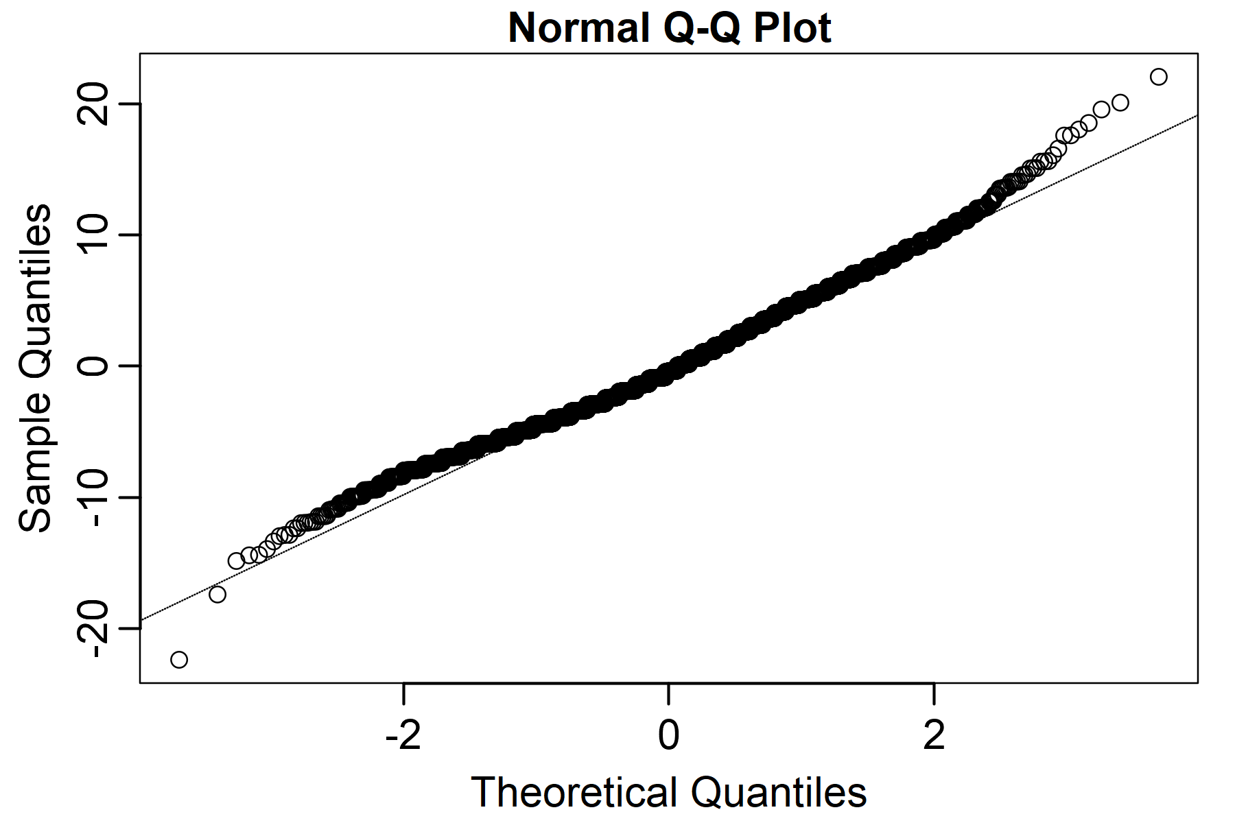
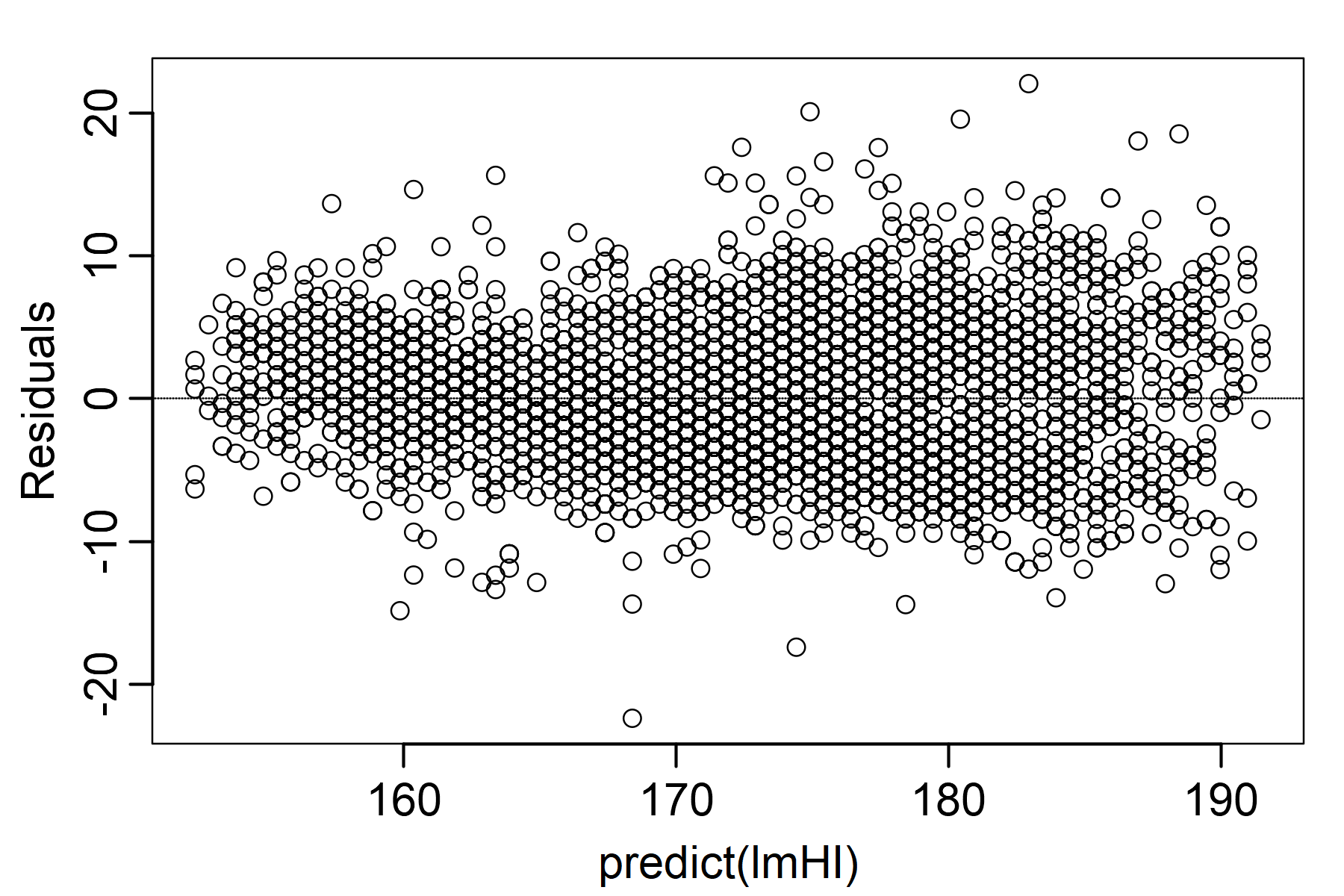
The QQ plot suggests the distribution of residuals is approximately normal (Figure 2.6 (a)), whereby the points lie approximately on a line. The plot of the residuals against the fitted values suggests linearity of residuals (Figure 2.6 (b)), whereby the points lie approximately on the horizontal line around the zero.
To jointly account for multiple criterion variables (and even for their interactions), a multiple regression model may be considered. The linear regression model assumes that the observed values of the dependent variable \(Y_p\) for respondent \(p\) can be predicted by a linear function of the values for a set of \(m\) observed predictors \(X_{p1}, \dots, X_{pm}\):
\[ Y_{p} = \beta_0 + \beta_1 X_{p1} + \dots + \beta_m X_{pm} + \epsilon_p, \tag{2.24}\]
with normally distributed, unbiased random errors \(\epsilon_p \sim \mathcal{N}(0, \sigma^2)\) independent for respondents \(p = 1, \dots, n\).
Interpretation of parameters is now slightly more complex. The \(\beta_0\) is now the mean expected value of the dependent variable \(Y_p\) when all predictors \(X_{pk}\) are zero. The slope \(\beta_k\) now reflects the mean change in the outcome \(Y_p\) associated with a unit increase of the predictor \(X_{pk}\) given that all other predictors remain constant. The model has the same assumptions as the simple linear regression model (linearity, independence, normality, and homoscedasticity of residuals), and again, these can be inspected visually using the diagnostic plots as presented above for the simple linear regression model.
Multiple regression in R. As an example, we present a final linear model considered in validation of the HCI (McFarland et al., 2017). This model provides proof of validity by demonstrating higher average scores for students majoring in science, similar to the \(t\) test used to compare average scores of undergraduate and graduate students in Section 2.3.3. But this model is more precise in that it also accounts for other characteristics of students and schools. More specifically, the model predicted the total test score (the dependent variable \(Y_p\)) of the HCIdata dataset by evaluating predictors including student gender (male, female, not specified), planned science major (yes/no coded as 1/0), study year, minority status (yes/no/not specified coded as min/maj/none), English as a first language (yes/no), and the school type (associate’s college AC, baccalaureate college with arts and sciences focus BCAS, research university R1, and master’s college or university MCU).
We fit a multiple regression model using the base lm() function. The anova() method computes an analysis of the variance table.
lmF <- lm(total ~ gender + major + factor(yearc5) + minority + EnglishF + typeSCH,
          data = HCIdata)
anova(lmF)
Analysis of Variance Table
Response: total
Df Sum Sq Mean Sq F value Pr(>F)
gender 2 260.7 130.36 13.2054 2.385e-06 ***
major 1 393.8 393.84 39.8952 4.947e-10 ***
factor(yearc5) 4 647.3 161.82 16.3920 8.300e-13 ***
minority 2 529.8 264.91 26.8346 6.291e-12 ***
EnglishF 1 319.7 319.72 32.3876 1.906e-08 ***
typeSCH 3 291.6 97.19 9.8449 2.339e-06 ***
Residuals 655 6466.0 9.87
---
Signif. codes: 0 '***' 0.001 '**' 0.01 '*' 0.05 '.' 0.1 ' ' 1The results suggest all predictors have a significant effect on the total score. A more detailed output is provided by the summary() method, including the estimated model parameters and significance of the differences from baseline levels in categorical variables.
summary(lmF)
Call:
lm(formula = total ~ gender + major + factor(yearc5) + minority +
    EnglishF + typeSCH, data = HCIdata)

Residuals:
    Min      1Q  Median      3Q     Max
-8.8708 -2.0195  0.1084  2.1314  7.3625

Coefficients:
                Estimate Std. Error t value Pr(>|t|)
(Intercept)      10.9021     0.5322  20.485  < 2e-16 ***
genderF          -0.8086     0.2597  -3.113 0.001931 **
gendernone       -2.2278     0.8311  -2.681 0.007536 **
major             1.2866     0.2657   4.842 1.60e-06 ***
factor(yearc5)2   2.0424     0.5102   4.003 6.96e-05 ***
factor(yearc5)3   1.1911     0.4951   2.406 0.016414 *
factor(yearc5)4   1.7943     0.5221   3.437 0.000626 ***
factor(yearc5)5   3.7029     0.5893   6.284 6.02e-10 ***
minoritymin      -1.5932     0.3258  -4.891 1.27e-06 ***
minoritynone     -2.2996     0.6276  -3.664 0.000268 ***
EnglishFno       -1.4160     0.3147  -4.499 8.07e-06 ***
typeSCHBCAS       0.2574     0.4056   0.635 0.525832
typeSCHR1         0.7349     0.3679   1.997 0.046193 *
typeSCHMCU       -1.3028     0.4205  -3.099 0.002028 **
---
Signif. codes:  0 '***' 0.001 '**' 0.01 '*' 0.05 '.' 0.1 ' ' 1

Residual standard error: 3.142 on 655 degrees of freedom
Multiple R-squared:  0.2742,    Adjusted R-squared:  0.2598
F-statistic: 19.04 on 13 and 655 DF,  p-value: < 2.2e-16
The test developers expected students planning to major in science and those from research universities R1 to score higher than average, which was confirmed by the model. On average, a student planning to major in science received a 1.29 point higher total score (out of 20) than their peers with the same characteristics but not planning to major in science. A student from a research university R1, on average, scored 0.73 points higher than their otherwise similar peer from an associate’s college. The model also confirmed lower scores for female students, students belonging to minorities, and English language learners, which was also supported by the existing research.
Other complexities of the regression model are possible. For example, in the HCI example, the students were nested in institutions and in classes, thus yielding a hierarchical structure. Other complexities may also come from the type of data being predicted, the data distributions involved, and the shape of the regression curve expected. We will be discussing regression models more deeply in the context of item functioning in Section 9.4.
In this section, we look closer at computational aspects of the parameter estimation. We first present the OLS method, based on minimization of RSS, already discussed in Section 2.3.6. We then describe an approach based on ML. These methods are illustrated on the simple linear regression model Equation 2.16.
To estimate the parameters \(\boldsymbol{\beta} = (\beta_{0}\), \(\beta_{1})\) in the linear regression model Equation 2.16 from the data, one may employ the OLS method: This includes minimization of the RSS with respect to parameters:
\[ \text{RSS}(\boldsymbol{\beta}) = \sum_{p = 1}^{n} \left(Y_{p} - \beta_{0} - \beta_{1} X_p\right)^2. \tag{2.25}\]
The graphical illustration provides intuitive explanation of the OLS method: The parameters \(\hat{\beta}_{i0}\) and \(\hat{\beta}_{i1} X_p\) are selected so that the total area of squares is as small as possible (Figure 2.7).
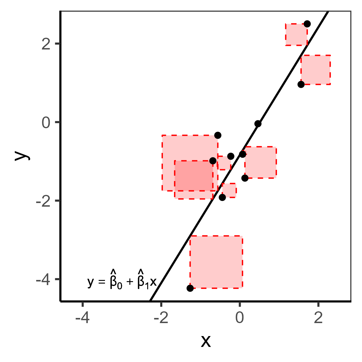
The resulting OLS estimates are item parameters \(\hat{\boldsymbol{\beta}} = (\hat{\beta}_{0}, \hat{\beta}_{1})\) which minimize the RSS in Equation 2.25, which is formally written as
\[ \hat{\boldsymbol{\beta}} = \arg\min_{\boldsymbol{\beta}} \text{RSS}(\boldsymbol{\beta}). \]
The minimized RSS for the OLS estimates is then
\[ \text{RSS}(\hat{\boldsymbol{\beta}}) = \sum_{p = 1}^{n} \hat{\epsilon}_{p}^2 = \sum_{p = 1}^{n} \left(Y_{p} - \hat{Y}_{p}\right)^2 = \sum_{p = 1}^{n} \left(Y_{p} - \hat{\beta}_{0} - \hat{\beta}_{1} X_p\right)^2. \]
The minimum of the RSS is obtained by setting its partial derivatives, with respect to item parameters, to zero and by solving the resulting system of estimating equations \(\frac{\text{RSS}}{\partial \beta_{0}} = 0\) and \(\frac{\text{RSS}}{\partial \beta_{1}} = 0\). The OLS method leads to the forms of parameter estimates Equation 2.18 already presented in Section 2.3.6 (for derivation see Exercise 2.5).
For estimation of item parameters, one may alternatively use the ML (maximum likelihood) method. Under the assumption of normal distribution of the residuals \(\epsilon_{p} \sim \mathcal{N}(0, \sigma^2)\) their mutual independence, and their independence on \(X_p\), the conditional distributions of dependent variables given the respondent’s value of independent variable are also normally distributed: \(Y_{p}| X_p \sim \mathcal{N}(\beta_{0} + \beta_{1} X_p, \sigma^2)\). Considering the form of the density for normal distribution \(\varphi\), see Equation C.4, the likelihood function, which describes the probability of the data given the parameters, has the following form:
\[ L(\boldsymbol{\beta}, \sigma) = \prod_{p = 1}^n \varphi(Y_{p}| X_p) = \prod_{p = 1}^n \frac{1}{\sqrt{2\pi\sigma^2}}\exp\left(-\frac{(Y_{p} - \beta_{0} - \beta_{1} X_p)^2}{2 \sigma^2}\right). \tag{2.26}\]
To obtain the MLE of item parameters \(\boldsymbol{\beta} = (\beta_{0}, \beta_{1})\), the likelihood function \(L(\boldsymbol{\beta})\) is maximized with respect to a set of parameters \(\boldsymbol{\beta}\) and the variance of \(\sigma^2\). To do so, the partial derivatives of the log-likelihood function, i.e., a logarithm of the likelihood function Equation 2.26, with respect to parameters are set to zero and the system of likelihood equations is solved (for derivation see Exercise 2.6). A logarithm is used because it is easier to find a maximum of the sum than a maximum of the product. The log-likelihood is given by
\[ l(\boldsymbol{\beta}, \sigma^2) = \log \left(\prod_{p = 1}^n \varphi(Y_{p}| X_p)\right) = - \frac{n}{2} \log\left(2\pi\right) - n \log\left(\sigma^2\right) - \frac{1}{2 \sigma^2}\sum_{p = 1}^n (Y_{p} - \beta_{0} - \beta_{1} X_p)^2. \]
Maximization of the log-likelihood \(l(\boldsymbol{\beta}, \sigma^2)\) with respect to item parameters \(\boldsymbol{\beta}\) once again reduces to the problem of minimization of \(\text{RSS} = \sum_{p = 1}^n (Y_{p} - \beta_{0} - \beta_{1} X_p)^2\). In other words, in this (special) case of simple linear regression and under the normality assumptions, the ML method leads to the same item parameter estimates \(\hat{\beta}_{0}\) and \(\hat{\beta}_{1}\) defined by Equation 2.18 as the OLS method.
More generally, for the multiple regression model Equation 2.24, the likelihood function has the form:
\[ L(\boldsymbol{\beta}, \sigma) = \prod_{p = 1}^n \varphi(Y_{p}| \boldsymbol{X}_p) = \prod_{p = 1}^n \frac{1}{\sqrt{2\pi\sigma^2}}\exp\left(-\frac{(Y_{p} - \boldsymbol{ X}_p\boldsymbol{\beta})^2}{2 \sigma^2}\right), \tag{2.27}\]
and the log-likelihood is then:
\[ l(\boldsymbol{\beta}, \sigma^2) = \log \left(\prod_{p = 1}^n \varphi(Y_{p}| \boldsymbol{X}_p)\right) = - \frac{n}{2} \log\left(2\pi\right) - n \log\left(\sigma^2\right) - \frac{1}{2 \sigma^2}\sum_{p = 1}^n (Y_{p} - \boldsymbol{X}_p\boldsymbol{\beta})^2, \tag{2.28}\]
where \(\boldsymbol{X}_p = (1, X_{p1}, \dots, X_{pm})\) is a vector of covariates of person \(p\) and \(\boldsymbol{\beta} = (\beta_0, \dots, \beta_m)^{\!\top}\) is a vector of model parameters.
In the case of multiple covariates, many of them may not be associated with the response variable. An important task is to select those variables which are important for prediction. The goodness of fit of competing models may be assessed by comparing their coefficient of determination \(R^2\) Equation 2.21, and significance of single covariates can be tested using the \(F\) statistic Equation 2.22 or the \(T\) statistic Equation 2.23 discussed in Section 2.3.6.2. In this section, we present further model selection and model fit criteria based on the likelihood function.
The likelihood-ratio test (LRT) can be used for comparing two models, one of which is a constrained version of the other. The submodel is typically defined by restricting to zero some of the parameters which are freely estimated under the larger model. The LRT is used to test the null hypothesis, specified by the restricted model \(M_{H_0}\), against the alternative, specified by the more general model \(M_{H_1}\). The test is based on the idea of assessing the goodness of fit via likelihood Equation 2.27 and using the ratio of the likelihoods given the observed data. If the constrained model is supported, the difference between the two likelihoods should be small, i.e., their ratio should be close to 1; in other words, the logarithm of the ratio should be close to 0. The LRT statistic is defined as:
\[ LR = -2\log \left(\frac{L(\hat{\boldsymbol{\beta}}_{H_0})}{L(\hat{\boldsymbol{\beta}}_{H_1})}\right), \]
where \(\hat{\boldsymbol{\beta}}_{H_1}\) and \(\hat{\boldsymbol{\beta}}_{H_0}\) are MLE of model parameters under the model \(M_{H_1}\) or under the submodel \(M_{H_0}\), respectively. The test statistic may also be expressed using the difference in log-likelihoods Equation 2.28 as:
\[ LR = -2 \left(l(\hat{\boldsymbol{\beta}}_{H_0}) - l(\hat{\boldsymbol{\beta}}_{H_1})\right). \tag{2.29}\]
Under the model \(M_{H_0}\), the \(LR\) statistic Equation 2.29 has an asymptotic \(\chi^2\)-distribution with as many degrees of freedom as the difference in the number of estimated parameters.
The goodness of fit of a model may be assessed by the Akaike information criterion (AIC) (Akaike, 1974)
\[ \mathrm{AIC} = 2k - 2 \log(L(\hat{\boldsymbol{\beta}})) \tag{2.30}\]
with \(L(\hat{\boldsymbol{\beta}})\) being the maximized likelihood function, and \(k\) being the number of estimated parameters used as a penalty. When comparing multiple models, the model with the lowest AIC value is the preferred one.
The Bayesian information criterion (BIC) (Schwarz, 1978) uses a different penalty for the number of parameters accounting for the sample size \(n\):
\[ \mathrm{BIC} = k \log(n) - 2 \log(L(\hat{\boldsymbol{\beta}})). \tag{2.31}\]
Once again, lower values of the BIC signal a better fitting model.
Model selection and model fit in R. To provide a practical example, we compare the final linear model lmF considered in validation of the HCI from Section 2.3.6.2 with a submodel without variable major. In R, the anova() function with argument test = "Chisq" may be used on two lm objects to test the submodel with LRT Equation 2.29. Alternatively, the lrtest() function of the lmtest package may be used, which provides more informative output.
lmFrestr <- lm(total ~ gender + factor(yearc5) + minority + EnglishF + typeSCH,
               data = HCIdata)
anova(lmFrestr, lmF, test = "Chisq")
Analysis of Variance Table
Model 1: total ~ gender + factor(yearc5) + minority + EnglishF + typeSCH
Model 2: total ~ gender + major + factor(yearc5) + minority + EnglishF +
typeSCH
Res.Df RSS Df Sum of Sq Pr(>Chi)
1 656 6697.5
2 655 6466.0 1 231.49 1.283e-06 ***
---
Signif. codes: 0 '***' 0.001 '**' 0.01 '*' 0.05 '.' 0.1 ' ' 1library(lmtest)Warning: package 'lmtest' was built under R version 4.5.2Loading required package: zoo
Attaching package: 'zoo'The following objects are masked from 'package:base':
as.Date, as.Date.numericlrtest(lmFrestr, lmF)Likelihood ratio test
Model 1: total ~ gender + factor(yearc5) + minority + EnglishF + typeSCH
Model 2: total ~ gender + major + factor(yearc5) + minority + EnglishF +
typeSCH
#Df LogLik Df Chisq Pr(>Chisq)
1 14 -1719.9
2 15 -1708.1 1 23.532 1.229e-06 ***
---
Signif. codes: 0 '***' 0.001 '**' 0.01 '*' 0.05 '.' 0.1 ' ' 1The submodel is rejected (\(LR = 23.5\), df = 1, p-value \(< 0.001\)). The conclusion of the LRT is consistent with the conclusion of the \(F\) test and of the \(t\) test performed in Section 2.3.6.2.
In R, the AIC() function may be used to extract the AIC Equation 2.30 from several objects including those returned by the lm() function. Here we compare the model lmF and a restricted model without variable major.
AIC(lmF, lmFrestr) df AIC
lmF 15 3446.188
lmFrestr 14 3467.719According to the AIC, the model lmF shows a better fit, whereas the AIC is lower.
The BIC() function might be used to extract the BIC Equation 2.31 for a set of models. We again compare model lmF and restricted model lmFrestr.
BIC(lmF, lmFrestr) df BIC
lmF 15 3513.774
lmFrestr 14 3530.800According to the BIC, model lmF is once more preferred over the restricted model, whereas the BIC is lower.
In Section 2.3.5, we discussed how correlation coefficients between the test score and the criterion variable may be used to support claims of test validity. In an applied setting, range restriction often occurs: A situation when only a restricted range of all possible values is observed and present in the data. For example, with admission tests, the test score (predictor \(X\)) is often used in the selection of future students. Depending on the restriction, the correlation estimate is deflated or inflated. To deal with range restriction, several corrections have been proposed, operating under a different set of assumptions. For the case of explicit or direct selection, i.e., when test score \(X\) is entirely leading the range restriction (e.g., only those with a score above some cut score are observed), Thorndike (1949) provides the following formula for correction of range restriction (see also Wiberg & Sundström, 2009):
\[ r^\star_{xy} = \frac{s^\star_x r_{xy}}{\sqrt{s^{\star2}_x r_{xy}^2 + s^2_x - s^2_x r_{xy}^2}}, \tag{2.32}\]
where \(r^\star_{xy}\) is the correlation estimate for the unrestricted sample, \(r_{xy}\) is the observed correlation between variables \(X\) and \(Y\) in the restricted sample, \(s_x\) is the estimated standard deviation of \(X\) in the restricted sample, and \(s^\star_x\) is the estimated standard deviation of \(X\) in the original sample.
A number of authors derived formula Equation 2.32 under different assumptions. Cohen (1955) provides the derivation of Equation 2.32 as the maximum likelihood estimate under the assumption of bivariate normal distribution. Gulliksen (1950, 11) provides reasoning for the formula under other sufficient assumptions, which are the same linear regression form of \(Y = \beta_0 + \beta_1 X + e\) with \(e \sim \mathcal{N}(0, \sigma^2_e)\), held in the complete as well as the restricted sample. The slope estimates Equation 2.18 then are
\[ b^\star_{1_{xy}} = \frac{s^\star_{xy}}{s^{\star2}_x} = \frac{s_{xy}}{s^2_x} = b_{1_{xy}}. \]
The same form of regression implies error \(e\) to be homoscedastic, i.e., the residual variance \(\sigma^2_e\) to be the same in the complete as well as the restricted sample, thus
\[ s^{\star2}_e = s^{\star2}_y(1 - r^{\star2}_{xy}) = s^2_y(1 - r^2_{xy}) = s^{2}_e. \]
These two conditions are sufficient for the formula Equation 2.32 to hold (Exercise 2.9).
Correction for range restriction in R. For demonstration purposes, let’s consider the following simulated example. We first generate a sample of 1,500 independent values (admission test scores) of normal variable \(X\) and values (subsequent study success score) of dependent variable \(Y\) from a normal distribution so that the correlation \(\text{Cor}(X, Y)\) is 0.729.
set.seed(987)
x <- rnorm(1500); e <- rnorm(1500); r <- 0.729
b1 <- r / sqrt(1 - r^2)
y <- b1 * x + e
cor(x, y)
[1] 0.7235678xvar <- x * 10 + 50
yvar <- y * 2.3 + 20
cor(xvar, yvar)[1] 0.7235678We see that the sample correlation between the 1,500 pairs of observations is 0.72, which is close to expected value. The variables are displayed in Figure 2.8 (a).
If students with a low test score \(X < 58\) were never admitted into the school, the future study success measured on scale 0 to 30 (dependent variable \(Y\)) would not be observed for these students (Figure 2.8 (b)). This would lead to lowering of the correlation coefficient when estimated from the restricted data in our simulated example from 0.72 to 0.36.
df <- data.frame(xvar, yvar)
# only admitted students with X > 58
admitted <- subset(df, xvar > 58)
cor(admitted$xvar, admitted$yvar)
[1] 0.3632685Using the formula Equation 2.32 we get a more realistic estimate of 0.65. For implementing the formula, we use the rangeCorrection() function of the psych package.
psych::rangeCorrection(r = cor(admitted$xvar, admitted$yvar),
                       sdu = sd(xvar), sdr = sd(admitted$xvar))
[1] 0.6547984However, note that the correlation may increase when removing the mid-range applicants (Figure 2.8 (c)).
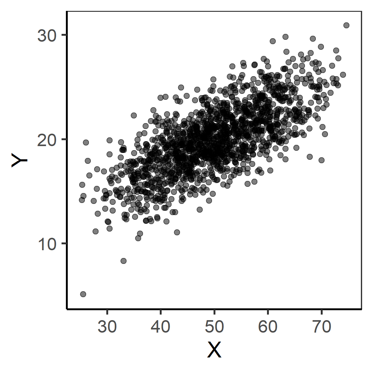
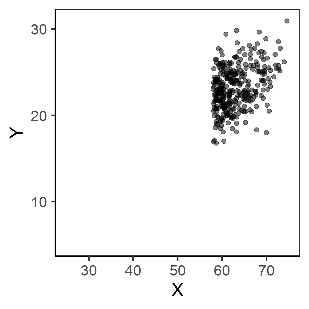
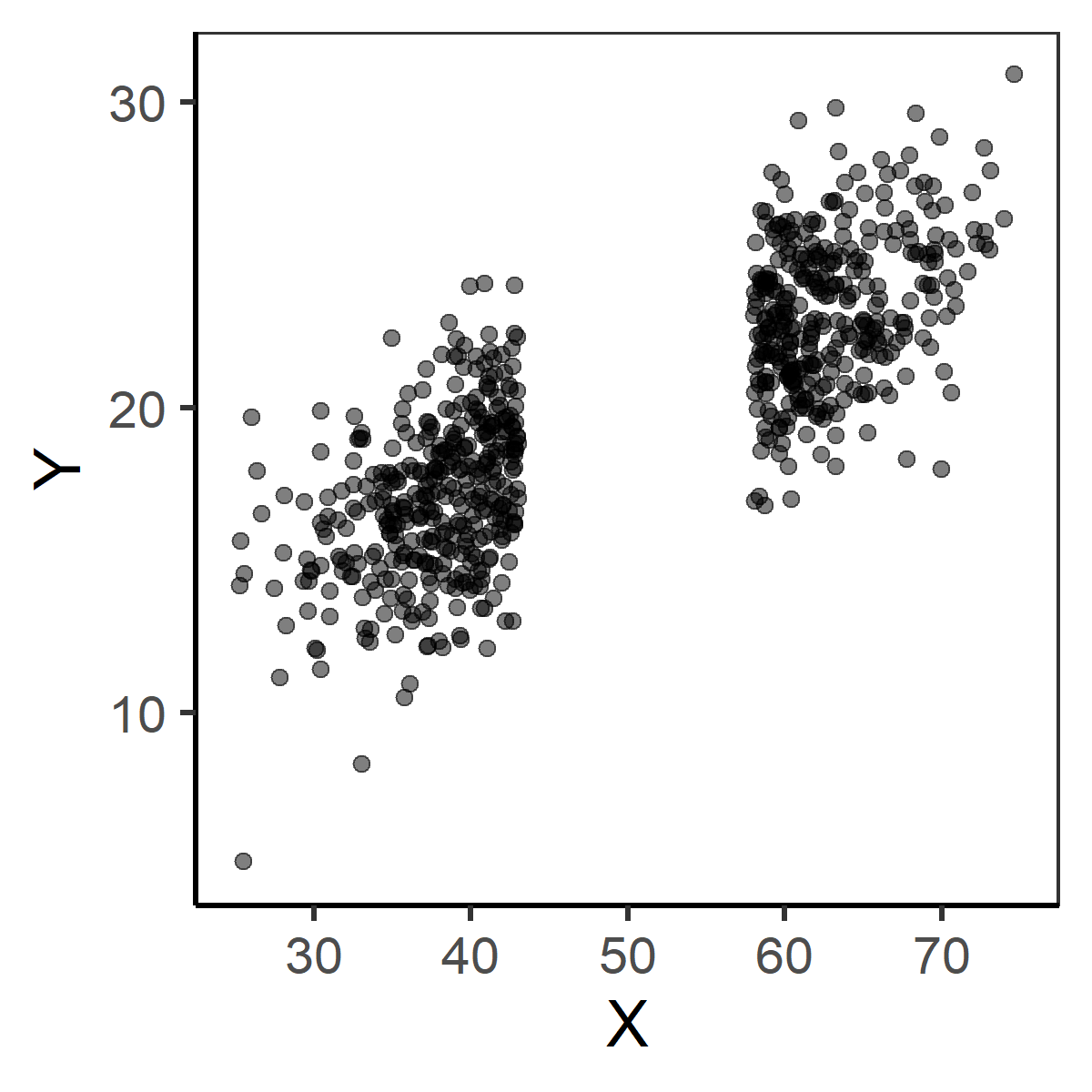
# only those above 58 or below 43 admitted
admitted2 <- subset(df, xvar > 58 | xvar < 43)
cor(admitted2$xvar, admitted2$yvar)
[1] 0.8127844psych::rangeCorrection(r = cor(admitted2$xvar, admitted2$yvar),
sdu = sd(xvar), sdr = sd(admitted2$xvar))[1] 0.7097014In this case the correlation estimated from restricted data is 0.81, while formula Equation 2.32 will provide an estimate of 0.71, close to the original value.
Under the section Validity, the ShinyItemAnalysis application offers methods for obtaining empirical proofs of test validity. The tab Criterion validity offers empirical proofs based upon a criterion, an external variable uploaded separately in the section Data.
Criterion validity. When a criterion variable is provided, either a boxplot or a scatter-plot, based upon the type of criterion variable, is displayed describing the relationship between the criterion variable and total scores (Figure 2.9). Furthermore, a correlation test for association between the criterion variable and total scores is offered.
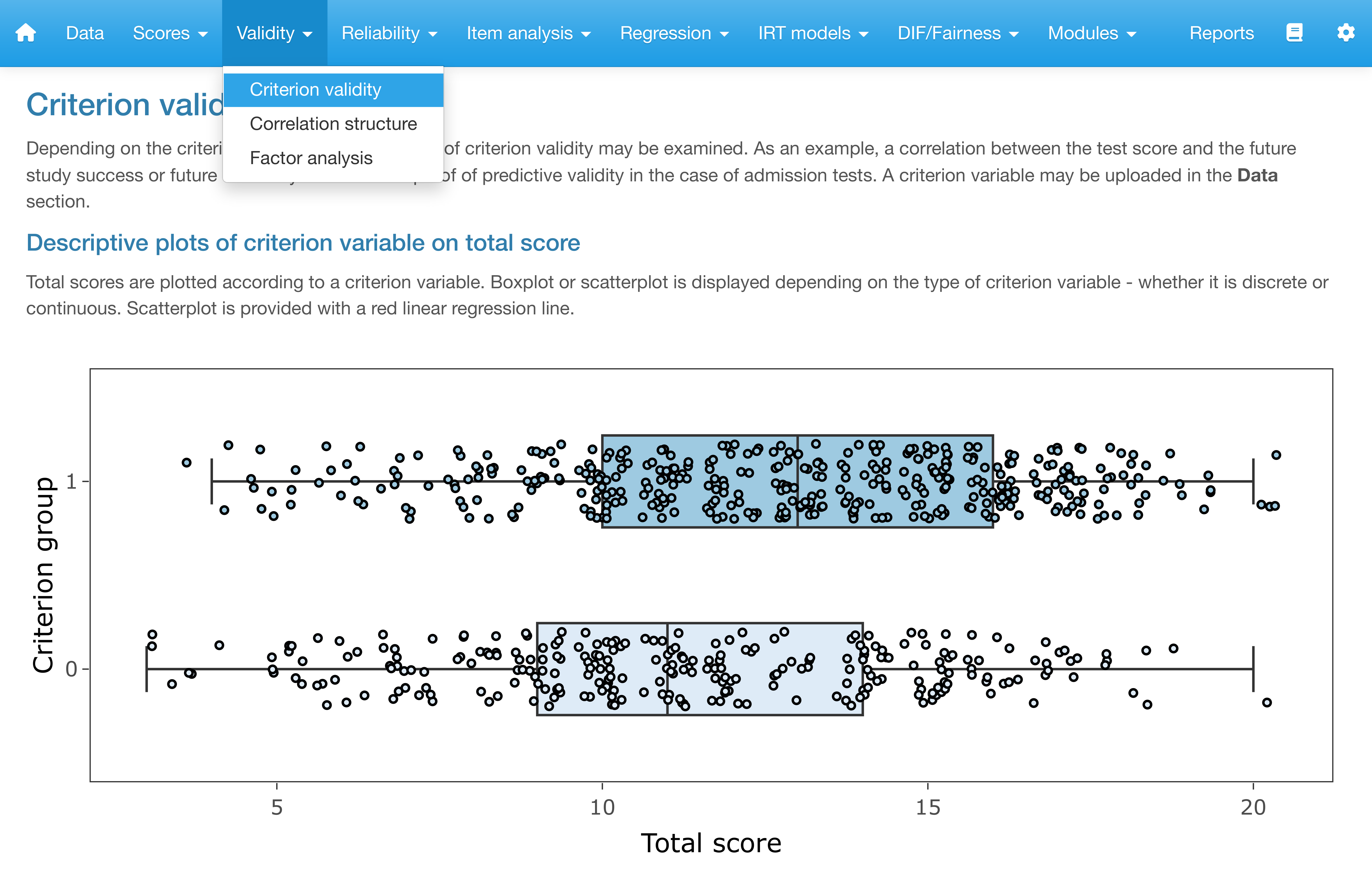
ShinyItemAnalysis.
In this chapter, we have discussed how to collect proofs of validity for a measurement instrument, based upon test content, and how to gain proofs of validity based on relationships to other, external variables. At the same time, we have presented classical statistical methods and their usage in the context of measurement validation. These included inferences based on ratios, \(t\) tests, ANOVA, correlation coefficients, and regression models. We have discussed two important methods for parameter estimation, which we will be returning to in the following chapters, the least-squares method and the maximum likelihood method. We have closed the methods part of the chapter by providing the corrected estimate of correlation under range restriction and by discussing how the range restriction may influence the validation process. Finally, we have presented how proofs of validity may be obtained with analyses available in the interactive ShinyItemAnalysis application. An obviously important part of the test validation has been omitted, analysis of the internal structure of the test. We will focus on this topic in the next chapter.