Appendix A — Introduction to R

This appendix provides an overview of R and RStudio, from installation through to data handling, graphics, and interactive applications with Shiny.

A.1 Installing R and RStudio

The language R is available on most operating systems. R for Windows, Mac and Linux can be downloaded directly from the project web page at https://www.r-project.org/. Go to the CRAN link and select your operating system.

RStudio is an integrated development environment (IDE) built specifically for R. We recommend that beginners in R use RStudio as it provides a structured environment with useful features such as code completion, integrated help, and project management. RStudio can be downloaded from https://posit.co/download/rstudio-desktop/. Note that prior to installing RStudio, R needs to already be installed on your computer.

A.2 Starting with R

A.2.1 R as a calculator

R can be used as a simple calculator. Type 2 + 2 in the R console and press Enter:

2 + 2

[1] 4

R uses standard arithmetic operators: + (addition), - (subtraction), * (multiplication), / (division), ^ (exponentiation), and %% (modulus).

5 * 3

[1] 15

10 / 4

[1] 2.5

2^10

[1] 1024

A.2.2 Assigning values to objects

In R, we can store values in objects using the assignment operator <-. The object can then be used later in calculations:

x <- 5
y <- 3
x + y

[1] 8

Object names can contain letters, numbers, dots, and underscores, but they must start with a letter or a dot (not followed by a number). R is case-sensitive, so myData and mydata are different objects.

A.2.3 Functions

Functions in R take arguments and return a result. For example, the sqrt() function calculates the square root:

sqrt(16)

[1] 4

Functions can have multiple arguments. The seq() function creates a sequence of numbers:

seq(from = 1, to = 10, by = 2)

[1] 1 3 5 7 9

To get help on a function, use ? followed by the function name:

?seq

A.2.4 Vectors

Vectors are the most basic data structure in R. They are created using the c() function (combine):

my_vector <- c(1, 4, 6, 7, 9)
my_vector

[1] 1 4 6 7 9

Many operations in R are vectorized:

my_vector * 2

[1]  2  8 12 14 18

my_vector + 10

[1] 11 14 16 17 19

You can access elements of a vector using square brackets:

my_vector[3]

[1] 6

my_vector[c(1, 3, 5)]

[1] 1 6 9

A.2.5 Data frames

Data frames are rectangular data structures where columns can be of different types. They are similar to spreadsheets or database tables:

my_df <- data.frame(
  name = c("Alice", "Bob", "Carol"),
  age = c(25, 30, 35),
  score = c(85.5, 92.3, 78.8)
)
my_df

   name age score
1 Alice  25  85.5
2   Bob  30  92.3
3 Carol  35  78.8

Columns can be accessed using the $ operator:

my_df$age

[1] 25 30 35

A.3 Installing packages

R packages extend the functionality of base R. Packages can be installed from CRAN using the install.packages() function:

install.packages("ggplot2")

Once installed, packages need to be loaded using library():

library(ggplot2)

Alternatively, you can call a function from a package without loading it using the :: operator:

ggplot2::ggplot()

To install a package from GitHub, you can use the remotes package:

install.packages("remotes")
remotes::install_github("username/packagename")

A.4 Data handling in R

A.4.1 Data types in R

R has several basic data types:

• Numeric: Real numbers (e.g., 3.14, 42)
• Integer: Whole numbers, specified with L suffix (e.g., 5L)
• Character: Text strings (e.g., "hello")
• Logical: Boolean values (TRUE or FALSE)
• Factor: Categorical variables

You can check the type of an object using class() or typeof():

x <- 3.14
class(x)

[1] "numeric"

y <- "hello"
class(y)

[1] "character"

z <- TRUE
class(z)

[1] "logical"

Factors are useful for categorical data:

gender <- factor(c("male", "female", "male", "female"))
gender

[1] male   female male   female
Levels: female male

levels(gender)

[1] "female" "male"  

Ordered factors preserve the ordering of categories:

education <- ordered(c("high school", "college", "graduate"), 
                     levels = c("high school", "college", "graduate"))
education

[1] high school college     graduate   
Levels: high school < college < graduate

A.4.2 Reading data

Data can be read from various file formats. The most common are CSV files:

my_data <- read.csv("data.csv")

For Excel files, the readxl package is useful:

library(readxl)
my_data <- read_xlsx("data.xlsx")

Data from R packages can be loaded using the data() function:

data("HCI", package = "ShinyItemAnalysis")
head(HCI, n = 3)

  Item 1 Item 2 Item 3 Item 4 Item 5 Item 6 Item 7 Item 8 Item 9 Item 10
1      1      1      1      1      1      0      0      1      1       1
2      1      1      1      1      1      1      0      1      1       1
3      1      1      1      1      0      1      0      1      1       1
  Item 11 Item 12 Item 13 Item 14 Item 15 Item 16 Item 17 Item 18 Item 19
1       1       1       1       1       0       1       0       1       1
2       1       1       1       1       1       1       1       1       1
3       1       1       1       1       0       1       1       1       1
  Item 20 gender major total
1       1      0     1    16
2       1      0     1    19
3       1      1     1    17

A.4.3 Wide vs. long format

Data can be organized in two main formats:

Wide format: Each item has its own column. This is how most psychometric data is stored.

# Wide format example
wide_data <- data.frame(
  id = 1:3,
  item1 = c(1, 0, 1),
  item2 = c(1, 1, 0),
  item3 = c(0, 1, 1)
)
wide_data

  id item1 item2 item3
1  1     1     1     0
2  2     0     1     1
3  3     1     0     1

Long format: Each row represents one observation (one person-item combination).

# Long format example
long_data <- data.frame(
  id = rep(1:3, each = 3),
  item = rep(paste0("item", 1:3), 3),
  response = c(1, 1, 0, 0, 1, 1, 1, 0, 1)
)
long_data

  id  item response
1  1 item1        1
2  1 item2        1
3  1 item3        0
4  2 item1        0
5  2 item2        1
6  2 item3        1
7  3 item1        1
8  3 item2        0
9  3 item3        1

You can convert between formats using the tidyr package:

library(tidyr)

# Wide to long
long_result <- pivot_longer(wide_data, cols = starts_with("item"), 
                            names_to = "item", values_to = "response")
head(long_result)

# A tibble: 6 × 3
     id item  response
  <int> <chr>    <dbl>
1     1 item1        1
2     1 item2        1
3     1 item3        0
4     2 item1        0
5     2 item2        1
6     2 item3        1

# Long to wide
wide_result <- pivot_wider(long_data, names_from = item, values_from = response)
wide_result

# A tibble: 3 × 4
     id item1 item2 item3
  <int> <dbl> <dbl> <dbl>
1     1     1     1     0
2     2     0     1     1
3     3     1     0     1

A.4.4 The tidyverse

The tidyverse is a collection of R packages designed for data science. Key packages include:

• dplyr: Data manipulation (filtering, selecting, mutating)
• tidyr: Data tidying (reshaping)
• ggplot2: Data visualization
• readr: Reading data files
• purrr: Functional programming
• stringr: String manipulation

library(tidyverse)

Common dplyr operations:

data("HCI", package = "ShinyItemAnalysis")

# Filter rows
HCI_high <- filter(HCI, total >= 15)
nrow(HCI_high)

[1] 202

# Select columns
HCI_items <- select(HCI, starts_with("Item"))
ncol(HCI_items)

[1] 20

# Create new variables
HCI <- mutate(HCI, pct_correct = total / 20 * 100)
head(HCI$pct_correct)

[1]  80  95  85 100  95 100

# Summarize data
summarize(HCI, mean_score = mean(total), sd_score = sd(total))

  mean_score sd_score
1   12.21198 3.639684

# Group and summarize
HCI |>
  group_by(gender) |>
  summarize(mean_score = mean(total), n = n())

# A tibble: 2 × 3
  gender mean_score     n
   <int>      <dbl> <int>
1      0       11.9   405
2      1       12.7   246

The pipe operator |> (or %>% from magrittr) allows you to chain operations:

HCI |>
  filter(total >= 10) |>
  group_by(gender) |>
  summarize(
    n = n(),
    mean_score = mean(total),
    sd_score = sd(total)
  )

# A tibble: 2 × 4
  gender     n mean_score sd_score
   <int> <int>      <dbl>    <dbl>
1      0   305       13.4     2.59
2      1   194       14.2     2.54

A.5 Graphics in R

R provides several systems for creating graphics. We describe the three most common: base R graphics, ggplot2, and lattice.

A.5.1 Base R graphics

Base R provides simple functions for common plots:

data("HCI", package = "ShinyItemAnalysis")
hist(HCI$total, main = "Histogram of HCI Total Scores",
     xlab = "Total Score", col = "lightblue")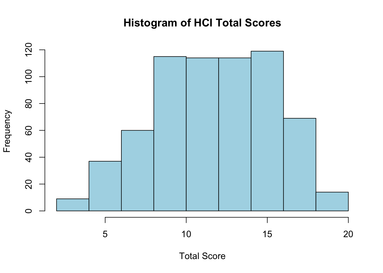

Figure A.1: Histogram of HCI total scores using base R graphics.

Other common base graphics functions include:

• plot(): Scatter plots and other basic plots
• boxplot(): Box plots
• barplot(): Bar plots
• lines(), points(): Add to existing plots

plot(HCI$total, HCI$"Item 1", xlab = "Total Score", ylab = "Item 1 Response",
     main = "Item 1 vs Total Score")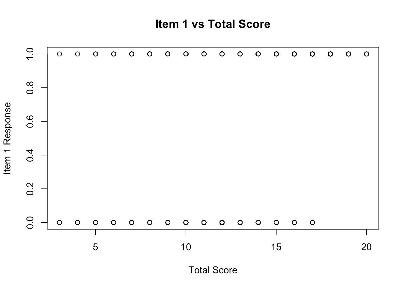

Figure A.2: Scatter plot example using base R graphics.

A.5.2 Graphics with the ggplot2 package

The ggplot2 package implements a grammar of graphics, building plots layer by layer:

library(ggplot2)

ggplot(HCI, aes(x = total)) +
  geom_histogram(binwidth = 1, fill = "steelblue", color = "white") +
  labs(title = "Histogram of HCI Total Scores",
       x = "Total Score", y = "Count") +
  theme_minimal()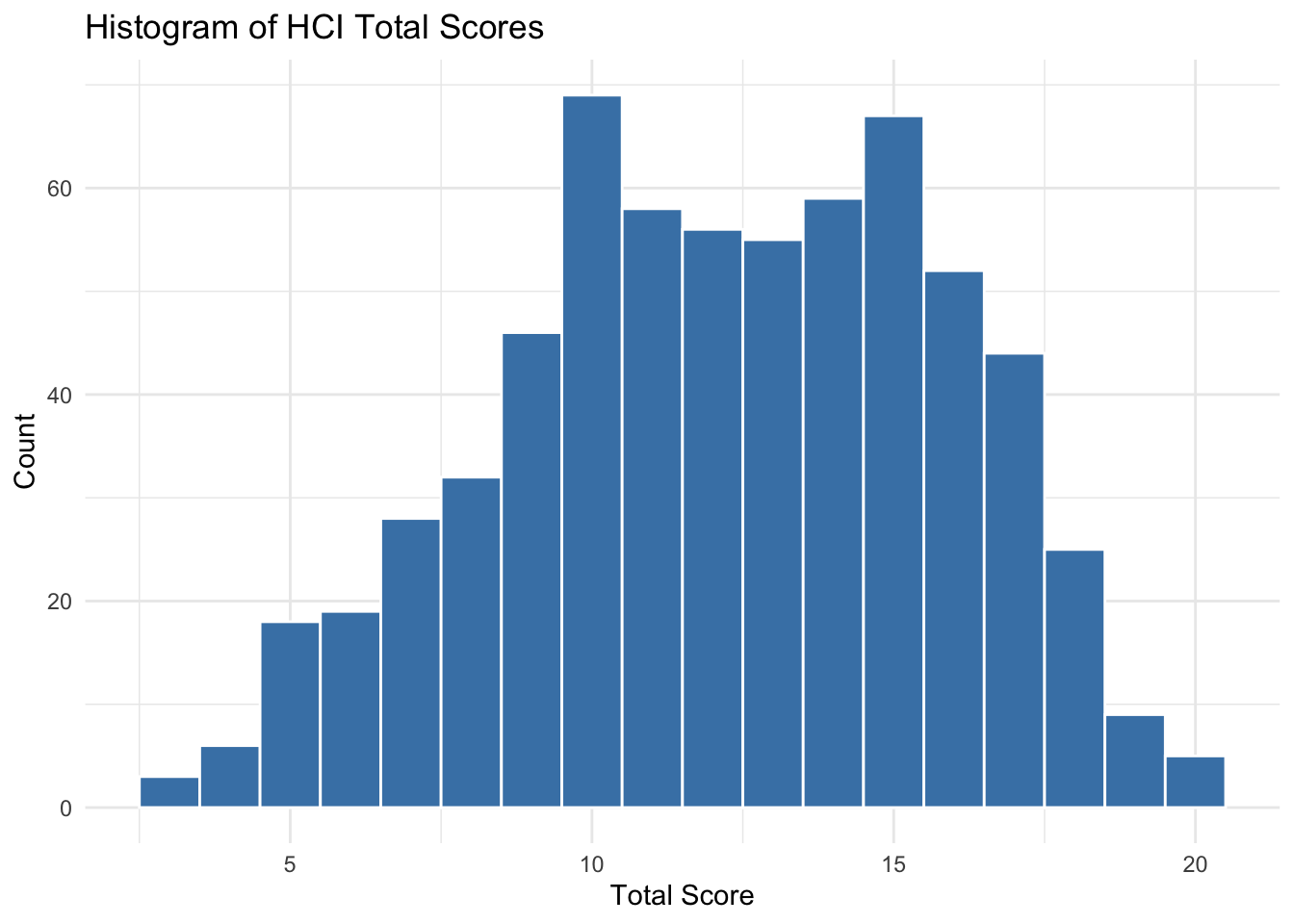

Figure A.3: Histogram of HCI total scores using ggplot2.

Key components of a ggplot:

• Data: The data frame to visualize
• Aesthetics (aes()): Mappings between data and visual properties
• Geometries (geom_*()): The type of plot (points, lines, bars, etc.)
• Scales: Control how data values map to visual properties
• Themes: Control appearance

More complex example with faceting:

ggplot(HCI, aes(x = total, fill = factor(gender))) +
  geom_histogram(binwidth = 1, alpha = 0.7, position = "identity") +
  facet_wrap(~ gender, labeller = labeller(gender = c("0" = "Male", "1" = "Female"))) +
  labs(title = "HCI Scores by Gender",
       x = "Total Score", y = "Count") +
  scale_fill_manual(values = c("0" = "#3498db", "1" = "#e74c3c"),
                    labels = c("Male", "Female"), name = "Gender") +
  theme_minimal()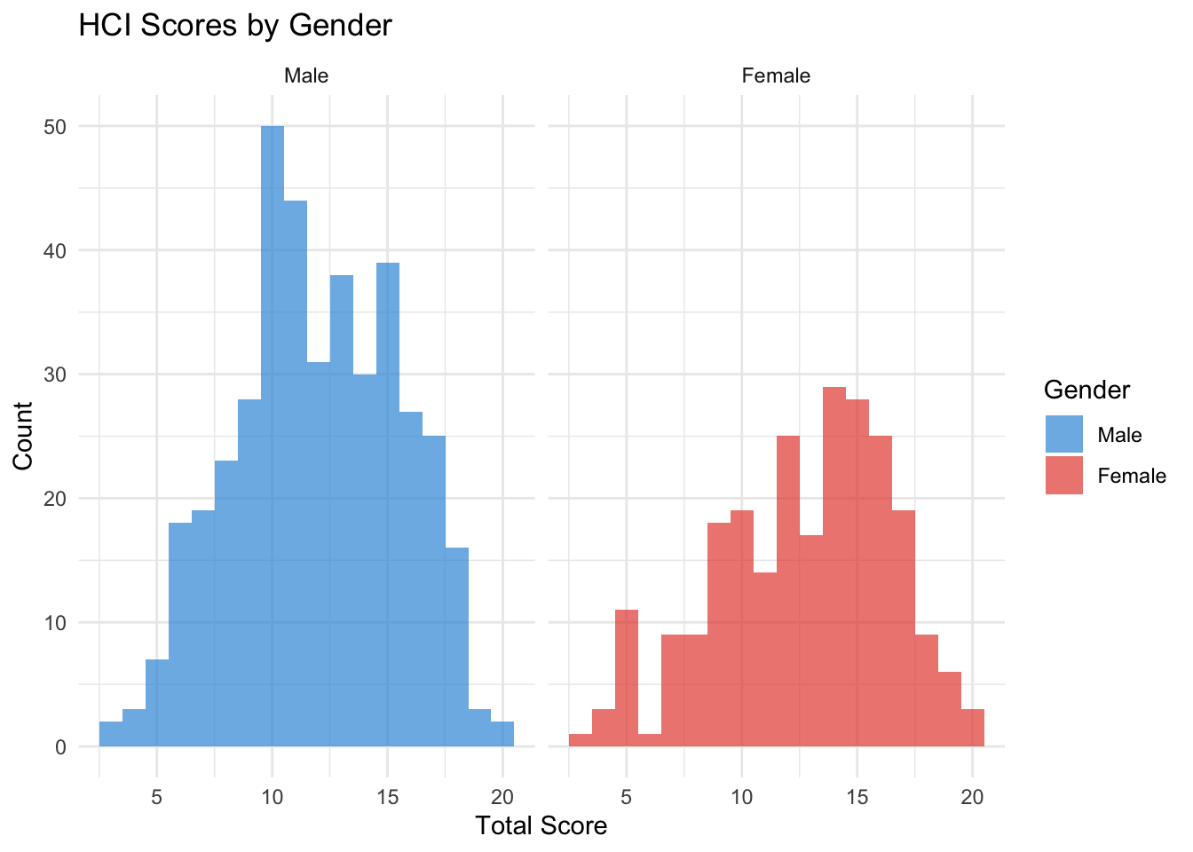

Figure A.4: Histogram of HCI total scores by gender using ggplot2.

A.5.3 lattice

The lattice package provides another approach to creating multi-panel graphics:

library(lattice)

histogram(~ total | factor(gender), data = HCI,
          xlab = "Total Score",
          main = "HCI Scores by Gender",
          layout = c(2, 1))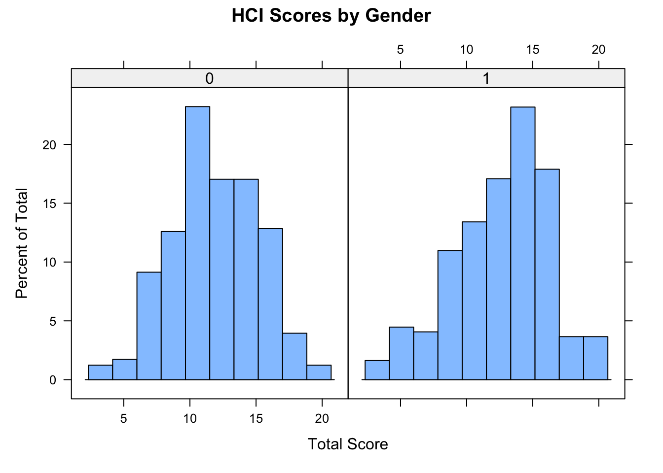

Figure A.5: Histogram of HCI total scores using lattice.

A.6 Interactive Shiny applications

Shiny is an R package for building interactive web applications. A basic Shiny app has two components:

• UI (User Interface): Defines the layout and appearance
• Server: Contains the logic and computations

Here is a minimal example:

library(shiny)

ui <- fluidPage(
  titlePane("Hello Shiny!"),
  sidebarLayout(
    sidebarPanel(
      sliderInput("n", "Number of observations:", 
                  min = 10, max = 500, value = 100)
    ),
    mainPanel(
      plotOutput("histogram")
    )
  )
)

server <- function(input, output) {
  output$histogram <- renderPlot({
    data <- rnorm(input$n)
    hist(data, main = "Random Normal Data", col = "steelblue", border = "white")
  })
}

shinyApp(ui = ui, server = server)

This app creates a histogram of random normal data where the user can control the sample size with a slider.

For more complex applications, see the ShinyItemAnalysis package which provides a comprehensive psychometric analysis Shiny application.

A.6.1 ShinyItemAnalysis package and its modules

The ShinyItemAnalysis package contains the interactive application, data, and functions for psychometric analysis. It also includes modules that demonstrate specific concepts.

ShinyItemAnalysis::run_app()