data(EPIA, package = "ShinyItemAnalysis")
head(EPIA, n = 2)
Item 1 Item 2 Item 3 Item 4 Item 5 score
1 96 36 80 78 79 369
2 42 2 1 1 1 47Traditional item analysis in Chapter 5 used ratios and correlation coefficients to estimate item difficulty and discrimination. To describe item functioning in more detail, the ratios of the correct answer or selected answer options were enumerated for ability groups defined by the total score and plotted out as an estimate of the ICC. While this empirical approach is simple and easy to implement even by hand, we discussed its limitations, including sample dependency: In samples of respondents with higher ability, the items may appear easier, while in lower ability samples, the items may appear more difficult. Similarly, in more heterogeneous samples, the same items might seem to better discriminate than when used in less heterogeneous samples of respondents.
In this chapter, we start building a more flexible approach in which the functioning of items will be modeled jointly for all levels of ability using a smooth function of a certain shape. The item difficulty, item discrimination, and other item properties will be defined by parameters of this function, describing its location or slope. Besides the low number of parameters needed to describe functioning of items across the whole ability continuum, the beauty and power of such a modeling approach also lies in the possibility to further extend the models in order to test for group differences and effects of other respondent characteristics, for effects of item type, or to account for more complex data structures such as hierarchical clustering of the respondents.
Various regression models may be used to describe item functioning and properties in more detail. The models typically predict the expected item score of person \(p\) on item \(i\) given their observed ability \(X_p\) and some set of item parameters \(\boldsymbol{\xi}_i\) which are to be estimated from data:
\[ \text{E} (Y_{pi}|X_p, \boldsymbol{\xi}_i) = f(X_p, \boldsymbol{\xi}_i). \tag{6.1}\]
The function \(f\) is specified by the researcher or practitioner to correspond with their beliefs about the item functioning and also to correspond to data types. Further extensions of the model are also possible. Especially, additional person or item characteristics may be considered as covariates besides observed ability \(X_p\).
Observed ability. Contrary to the IRT models presented in the next chapter, the trait or ability here is considered to be an observed value \(X_p\), which is assumed to be directly available and does not need to be estimated. This greatly simplifies presentation of the methods and estimation techniques. As an example, consider the case of the HeightInventory dataset in which the respondent’s height was assessed with a questionnaire and the respondent’s height was measured in centimeters. The questionnaire item properties can then be assessed with respect to the respondent’s observed measurable height.
In educational, psychological, and health-related measurements, a precise measure of respondent’s ability is rarely available at hand. Instead, the standardized total score or the total score is used as the simplest observed ability. While this approach is well rooted in psychometric research (see, for example, Swaminathan & Rogers, 1990), note that non-zero predicted item score \(\hat{Y}_{pi}\) may be obtained for zero total score \(X_p = 0\) due to model imprecision.
Other, concurrent representations of observed ability \(X_p\) may also be used in the regression model Equation 6.1 to describe item functioning in terms of criterion validity discussed in Chapter 2. Examples of these are a total score from a different test measuring the same construct or a score from an earlier administration of the same test.
Throughout the next sections, we mostly assume the observed ability to be a continuous variable, which corresponds to the case of IRT models (presented in Chapter 7 and Chapter 8) when ability is unobserved. However, models for binary, ordinal, or categorical abilities may also be of interest.
Models for different item types. In the following sections of this chapter, we will present various choices of the function \(f\) in Equation 6.1 which define regression models appropriate for different types of assessment data: When the item score is continuous, or at least can be treated as such, a linear regression model may be used with \(f\) being a linear function; this model was already discussed in Section 9.4. In this chapter, we introduce other regression models: In educational or psychological assessment, dichotomous (e.g., true/false) items are more common, for which the generalized linear model (GLM) such as the logistic or the probit (normal-ogive) regression models are a typical choice, using logit or probit \(f\) respectively. Extensions of these are nonlinear models which are able to account for the respondent’s guessing or inattention when answering. Psychological and health-related measurements often employ Likert-scale assessments with ordinal items, for which some of the ordinal regression models can be used, such as the cumulative logit model or the adjacent-categories logit model. Finally, to describe functioning of the multiple-choice items, the multinomial regression model can be employed.
One or more models. Note that model Equation 6.1 may be applied on data on a single item \(i\). This approach may be repeated for all items to obtain parameter estimates of the whole instrument. This approach is more feasible, especially for instruments with different item formats in which sets of estimated parameters (and number of parameters) may differ for different items.
Model Equation 6.1 may also be fitted for all items \(i = 1, \dots, m\) jointly. The response pattern \(\boldsymbol{Y}_p = (Y_{p1}, \dots, Y_{pm})\) is then modeled as a function of the observed ability \(X_p\) and set of item parameters \(\boldsymbol{\xi}\):
\[ \text{E} (\boldsymbol{Y}_{p}|X_p, \boldsymbol{\xi}) = f(X_p, \boldsymbol{\xi}). \tag{6.2}\]
We will discuss the joint model in more detail in Section 6.8. For the rest of the chapter we will mostly focus on the description of a single item using the model Equation 6.1.
The linear regression model, which is appropriate for a case of continuous items, is the simplest regression model. We start with this model mainly for pedagogical reasons, acknowledging that continuous items are not typical for educational, psychological, or health-related measurement instruments.
Functioning of continuous items can be analyzed using the linear regression model:
\[ \text{E}(Y_{pi} | X_p, \boldsymbol{\xi}_i) = \beta_{i0} + \beta_{i1} X_p. \]
In this special case of model Equation 6.1, the expected score on item \(i\) by person \(p\) is assumed to be a linear function of the respondent’s observed ability \(X_p\), a so-called linear predictor \(f(X_p) = \beta_{i0} + \beta_{i1} X_p\). The linear model can be alternatively presented in the form of Equation 2.16, already discussed in Chapter 2:
\[ Y_{pi} = \beta_{i0} + \beta_{i1} X_p + \epsilon_{pi}, \tag{6.3}\]
where \(\epsilon_{pi}\) is a random error, which is assumed to have a zero mean and some positive variance \(\sigma^2_i\) and to be uncorrelated with the observed ability \(X_p\).
The unknown parameters \(\boldsymbol{\xi}_i\), in this case the set of parameters \(\beta_{i0}\), \(\beta_{i1}\), and \(\sigma^2_i\), are to be estimated based upon the data; see Section 6.5 for details. The first of these parameters, \(\beta_{i0}\) is the intercept, describing the expected item score for a respondent with an observed ability of zero \(X_p = 0\). The second parameter \(\beta_{i1}\) is the slope, describing the expected increase in the item score \(Y_{pi}\) with every unit increase in \(X_p\).
Item functioning with the linear regression model in R. To provide a practical example, let us consider the continuous EPIA dataset.
data(EPIA, package = "ShinyItemAnalysis")
head(EPIA, n = 2) Item 1 Item 2 Item 3 Item 4 Item 5 score
1 96 36 80 78 79 369
2 42 2 1 1 1 47We will first consider the observed ability to be the total score, calculated for each respondent as the sum of their item scores, provided by variable score. The first respondent has a total score of 369, while the second respondent only has a total score of 47.
Another variable to consider as the observed ability is the standardized total score (the Z-score). As introduced in Chapter 1, the Z-score Equation 1.1 is calculated by subtracting the sample mean and dividing the result by a sample standard deviation; in R this can be easily calculated by hand or by using the scale() function.
EPIA$zscore <- scale(EPIA$score)For respondents in the EPIA dataset, the average total score is 251.90, and the SD is 92.60. The Z-score of the first respondent is 1.26; i.e., their level of anxiety was 1.26 SD above the average score. The Z-score of the second respondent is \(-2.21\); i.e., their level of anxiety was 2.21 SD below the average.
Below, we fit a linear model using the base lm() function to estimate the mean score of item 1, “Longs for excitement”, given the total score of the whole test. We save the output as the fitLM. The model summary then provides estimated coefficients and their significance, overall model fit in terms of \(R^2\), and summary statistics of residuals.
summary(fitLM <- lm(`Item 1` ~ score, data = EPIA))
Call:
lm(formula = `Item 1` ~ score, data = EPIA)

Residuals:
    Min      1Q  Median      3Q     Max
-95.461 -15.981  -0.639  17.072  69.689

Coefficients:
             Estimate Std. Error t value Pr(>|t|)
(Intercept) 15.529298   2.167765   7.164 1.49e-12 ***
score        0.187777   0.008078  23.246  < 2e-16 ***
---
Signif. codes:  0 '***' 0.001 '**' 0.01 '*' 0.05 '.' 0.1 ' ' 1

Residual standard error: 24.03 on 1031 degrees of freedom
Multiple R-squared:  0.3439,    Adjusted R-squared:  0.3433
F-statistic: 540.4 on 1 and 1031 DF,  p-value: < 2.2e-16
The model explains about 34% of the variability of the item scores, as can be read from the R-squared statistics. The model suggests that a respondent with a zero total score \(X_p\) has an average score of 15.53 on this item, the difference from a zero point score being due to model imprecision. With each total score point, the average item score rises by 0.19 points (also see Figure 6.1 (a)).
Estimates of the model parameters may be extracted separately with the coef() method, and their standard errors may be printed out using the vcov() method which displays the variance/covariance matrix; its diagonal provides squared standard errors.
coef(fitLM)(Intercept) score
15.5292976 0.1877769 sqrt(diag(vcov(fitLM)))(Intercept) score
2.167765243 0.008077792 We further fit the same model on a Z-score instead of the total score. We again use the lm() function to fit the linear model. As expected, the model fit is exactly the same as previously (see Supplementary R code for the model summary). We display the coefficients using the coef() method.
coef(lm(`Item 1` ~ zscore, data = EPIA))(Intercept) zscore
62.82962 17.38755 The interpretation of item parameters can now be completed with respect to the population mean score. The model predicts that a respondent with a Z-score of 0, hence with a total score equal to a sample mean of 251.90, has an average score of 62.83 on item 1. With each increase of the Z-score by one unit, i.e., increasing the original total score by one standard deviation (92.60 points), the average score on item 1 increases by 17.39 points.
Considering Equation 2.18, the relationship between the estimated model parameters and the traditional item parameters – item difficulty measured by mean item score and item discrimination measured by correlation between item score and Z-score – is as follows: The intercept \(\beta_{i0}\) corresponds to the average item score, and the slope \(\beta_{i1}\) corresponds to the correlation between item score and Z-score multiplied by standard deviation of item score:
mean(EPIA$`Item 1`)[1] 62.82962cor(EPIA$`Item 1`, EPIA$zscore) * sd(EPIA$`Item 1`) [,1]
[1,] 17.38755Regression lines for the two models are plotted with the ggplot() function of the ggplot2 package (see Supplementary R code).
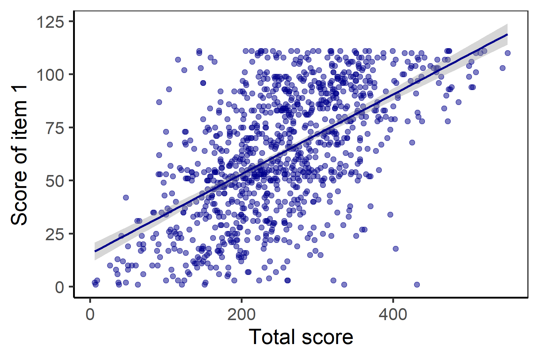
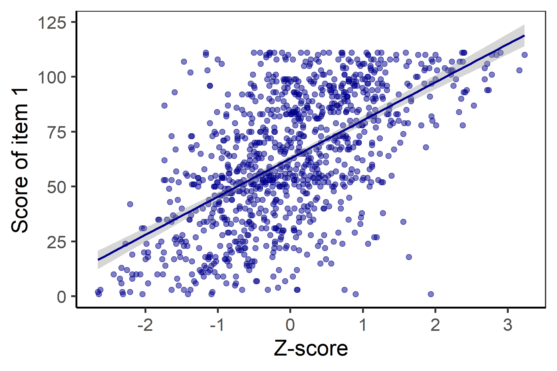
EPIA dataset.
Note that the two models are equivalent (Figure 6.1), with the main difference being the x-axis with respect to how the model is interpreted. To avoid the imprecise interpretation for the intercept in terms of a zero-point total score, and to provide interpretation closer to the IRT models presented in Chapter 7 and Chapter 8, we will be further fitting the regression models presented in the following sections with respect to the Z-scores.
Binary items are typical for both educational and psychological measurements. They include the true/false items for checking a respondent’s knowledge, or agree/disagree items for assessing a respondent’s attitudes or health status. In binary items, responses are typically rated as \(1\) for true/correct/endorsement and \(0\) otherwise. The expected item score (given the ability \(X_p\)) is therefore equal to the probability of a correct response (given \(X_p\)), which we further denote \(\pi_{pi}\):
\[ \pi_{pi} \coloneqq \text{E}(Y_{pi} | X_p) = \text{P}(Y_{pi} = 1|X_p). \]
A logistic regression model estimates the probability of the correct answer \(\pi_{pi}\) on binary item \(i\) for a respondent \(p\) with ability \(X_p\) by an S-shaped logistic curve:
\[ \pi_{pi} = \frac{\exp(\beta_{i0} + \beta_{i1} X_p)}{1 + \exp(\beta_{i0} + \beta_{i1} X_p)}. \tag{6.4}\]
The parameter \(\beta_{i0}\) describes a horizontal location of the fitted curve and the parameter \(\beta_{i1}\) describes a curve’s slope.
With the logistic regression model Equation 6.4, a specific function of the probability \(\pi_{pi}\) called logit is a linear function of the observed ability \(X_p\):
\[ g(\pi_{pi}) = \text{logit}(\pi_{pi}) = \log\left(\frac{\pi_{pi}}{1 - \pi_{pi}}\right) = \beta_{i0} + \beta_{i1}X_p, \tag{6.5}\]
which is an equivalent definition of the model Equation 6.4.
In expression Equation 6.5, the ratio of the probability of answering an item correctly to the probability of answering it incorrectly is termed as the odds of answering the item correctly. The logit is the logarithm of the odds (also called the log-odds) of answering item \(i\) correctly.
The intercept \(\beta_{i0}\) is then the log-odds of answering item \(i\) correctly for a respondent with a zero observed ability:
\[ \text{logit}(\text{P}(Y_{pi} = 1|X_p = 0)) \coloneqq \log\left(\frac{\text{P}(Y_{pi} = 1|X_p = 0)}{\text{P}(Y_{pi} = 0|X_p = 0)}\right) = \beta_{i0}. \]
The slope \(\beta_{i1}\) is the log-odds ratio by which the log-odds of answering an item correctly would increase with a unit increase in ability level:
\[ \begin{split} \beta_{i1} &= (\beta_{i0} + \beta_{i1}(x + 1)) - (\beta_{i0} + \beta_{i1}x)\\ &= \text{logit}(\text{P}(Y_{pi} = 1|X_p = x + 1)) - \text{logit}(\text{P}(Y_{pi} = 1|X_p = x)) \\ &= \log\left(\frac{\frac{\text{P}(Y_{pi} = 1|X_p = x + 1)}{\text{P}(Y_{pi} = 0|X_p = x + 1)}}{\frac{\text{P}(Y_{pi} = 1|X_p = x)}{\text{P}(Y_{pi} = 0|X_p = x)}}\right). \end{split} \]
As it includes two parameters, model Equation 6.4 is sometimes referred to as a 2PL model.
Item functioning with the logistic regression model in R. We demonstrate the model estimation in R and the interpretation of parameters in the logistic regression model Equation 6.4 with the binary HCI dataset and its item number 13. We first compute the Z-scores by standardizing the total scores (variable total) with the scale() function. The logistic model is then fitted using the glm() function with an argument family = binomial, referring to the binomial distribution of binary data. Similar to before, the summary() method can be used to display the summary of the fitted model fit_2PL (see Supplementary R code).
data(HCI, package = "ShinyItemAnalysis")
zscore <- scale(HCI$total)
fit_2PL <- glm(HCI[, 13] ~ zscore, family = binomial)
We display estimated coefficients with the coef() method. The vcov() method can be used to display the variance/covariance matrix; its diagonal is extracted with the diag() function which provides squared standard errors.
coef(fit_2PL)(Intercept) zscore
0.5552228 1.1824314 sqrt(diag(vcov(fit_2PL)))(Intercept) zscore
0.09322431 0.10836769 The estimated intercept \(\beta_{i0} = 0.56\) (SE = 0.09) is the log-odds of answering item 13 correctly for a respondent with a Z-score of 0 points (i.e., respondent with an average total score). In other words, an average respondent would have a probability of \(\frac{\exp( 0.56)}{1 + \exp( 0.56)}\) = 0.64 of answering item 13 correctly. With each standard deviation increase in the total score (i.e., each one-point increase in the Z-score), the log-odds of answering item 13 correctly would increase by the ratio of \(\beta_{i1} = 1.18\) (SE = 0.11). For a respondent with a Z-score of 1 (i.e., total score 1 standard deviation above average), the log-odds of answering the item correctly would thus be \(0.56 + 1.18 = 1.74\), and the probability of answering item 13 correctly would be \(\frac{\exp(0.56 + 1.18)}{1 + \exp(0.56 + 1.18)} = 0.85\) (Figure 6.2).
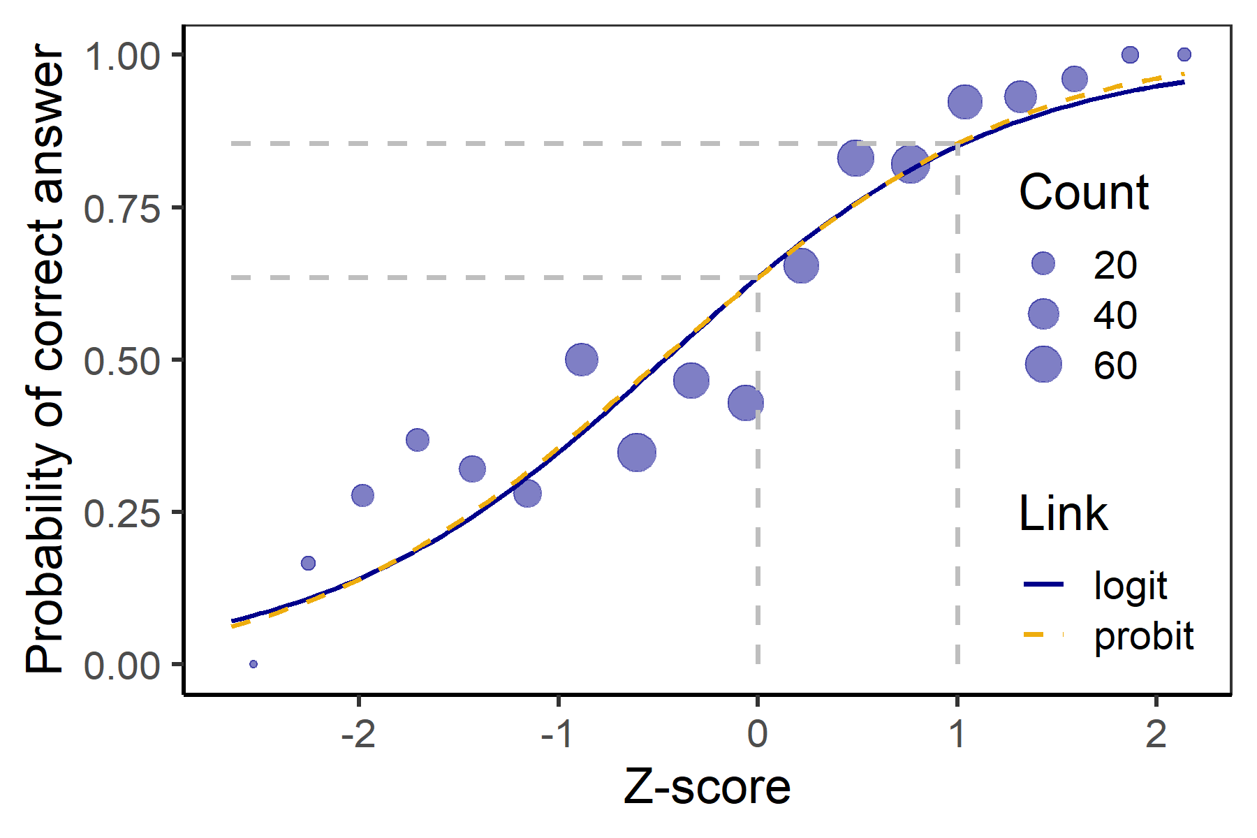
HCI dataset. Gray dashed lines highlight probabilities for respondents with the Z-score of 0 and 1.
The logistic regression model Equation 6.4 belongs to a wider class of GLMs. In the linear model Equation 6.3, the mean response \(\text{E}(Y_{pi}|X_p)\) is predicted by the linear term \(\beta_{i0} + \beta_{i1} X_p\), while in the GLM the mean response depends upon this linear predictor through link function \(g\), which satisfies
\[ \text{E}(Y_{pi}|X_p) = g^{-1}(\beta_{i0} + \beta_{i1}X_p). \]
A number of commonly used link functions exists. Their usage options are determined by several considerations, including the type and distribution of the data. For normally distributed data, the link function \(g\) is the identity function, leading to linear regression model Equation 6.3. For other data types, a higher number of possible link functions exists, but there is always a well-defined so-called canonical link function which is derived from the density function and has pleasant properties. For binary data, the canonical link is the logit function discussed above, i.e., logarithm of odds from Equation 6.5, which gives a name to the model – logistic regression.
Other link functions \(g\) are possible as well. A popular alternative is the probit link function, which is the inverse of the CDF of the standard normal distribution, \(\Phi^{-1}\). The probit regression model is thus defined as
\[ g(\pi_{pi}) = \textrm{probit}(\pi_{pi}) = \Phi^{-1}(\pi_{pi}) = \beta_{i0} + \beta_{i1}X_p. \tag{6.6}\]
The intercept parameter \(\beta_{i0}\) is related to the probability of answering item \(i\) correctly for an average respondent, i.e., for a respondent with zero observed ability:
\[ \beta_{i0} = \Phi^{-1}(\text{P}(Y_{pi} = 1 | X_p = 0)). \]
The slope \(\beta_1\) describes the change in probit index associated with a unit increase in ability level:
\[ \beta_{i1} = \Phi^{-1}(\text{P}(Y_{pi} = 1 | X_p = x + 1)) - \Phi^{-1}(\text{P}(Y_{pi} = 1 | X_p = x)). \]
The probability of a correct answer in item \(i\) by person \(p\) is then the inverse of the probit, i.e., the CDF of the standard normal distribution Equation C.4:
\[ \pi_{pi} = \Phi(\beta_{i0} + \beta_{i1}X_p). \tag{6.7}\]
The popularity of this non-canonical link function may be for historical reasons as well as for computational purposes as the values of the CDF were tabulated years ago and thus they were easy to apply without computers.
Probit regression model in R. In the glm() function, the logit link function Equation 6.5 is the default option for the binomial family. To use other link functions, an argument link needs to be specified. Here we illustrate fitting the probit regression model Equation 6.6 for item 13 of the HCI dataset.
fit_2PL_prob <- glm(HCI[, 13] ~ zscore, family = binomial(link = "probit"))We print estimated parameters and standard errors.
coef(fit_2PL_prob)(Intercept) zscore
0.3439692 0.7122449 sqrt(diag(vcov(fit_2PL_prob)))(Intercept) zscore
0.05488826 0.06081546 For item 13, the intercept is estimated at 0.34 (SE = 0.05), and the slope is estimated at 0.71 (SE = 0.06).
We will use the pnorm() function which enumerates the cumulative distribution function of the normal distribution to further interpret the parameter estimates. As before, we will calculate the probability of answering item 13 correctly for a respondent with the Z-score of 0, and for a respondent with the Z-score of 1:
pnorm(coef(fit_2PL_prob)[1])(Intercept)
0.6345653 pnorm(coef(fit_2PL_prob)[1] + coef(fit_2PL_prob)[2])(Intercept)
0.8545648 In this case, the probability of a correct answer to item 13 by a respondent with an average observed ability (Z-score of 0) is estimated as \(\Phi(0.34) = 0.63\). For a respondent with a Z-score of 1 (i.e., with a total score 1 standard deviation above the average), the probability of answering item 13 correctly would be \(\Phi(0.34 + 0.70) = 0.85\). Both predictions are very similar to predictions obtained before with logistic regression model Equation 6.4.
The fitted logistic and probit regression curves can be displayed with the ggplot() function of the ggplot2 package (see Supplementary R code). The proximity of the logistic and probit regression models is very close (Figure 6.2).
Note that the ratio between the discrimination parameters estimated by the logistic regression model Equation 6.4 and the probit regression model Equation 6.7 is approximately \(\frac{\hat{\beta}_{i1 \textrm{logit}}}{\hat{\beta}_{i1 \textrm{probit}}} = \frac{1.16}{0.70} = 1.65 \doteq 1.7\). In the framework of the IRT models, this ratio is oftentimes denoted as a multiplication coefficient \(D \doteq 1.7\). We will get back to this coefficient in the context of IRT models in Chapter 7.
To obtain a better interpretation of item parameters, it may be convenient to re-parametrize the logistic regression model Equation 6.4. Instead of the classical linear predictor \(\beta_{i0} + \beta_{i1} X_p\), the linear predictor is defined as \(a_i(X_p - b_i)\), with a new set of parameters \(a_i\) and \(b_i\), which is typical in IRT models. The logistic regression model then takes the form:
\[ \pi_{pi} = \frac{\exp(a_i(X_p - b_i))}{1 + \exp(a_i(X_p - b_i))}. \tag{6.8}\]
Interpretation of the parameters is displayed in Figure 6.3. In this form of the model, parameter \(b_i\) describes the difficulty of item \(i\), which is now nicely interpretable as the location of the inflection point, and as the ability needed to correctly answer (or endorse) the item with 50% probability:
\[ \text{P}(Y_{pi} = 1 | X_p = b_i) = \frac{\exp\left(a_i(b_i - b_i)\right)}{1 + \exp\left(a_i(b_i - b_i)\right)} = \frac{\exp (0)}{1 + \exp (0)} = \frac{1}{2}. \]
Parameter \(a_i\) describes the discrimination of item \(i\), the slope at inflection point. This can be seen when we take a derivative of the probability function and evaluate it at the inflection point \(b_i\):
\[ \left.\frac{\partial \pi_{pi}}{\partial X_p}\right\vert_{X_p = b_i} = \left.\frac{a_i \exp\left(a_i(X_p - b_i)\right)}{\left[ 1 + \exp\left(a_i(X_p - b_i)\right) \right]^2}\right\vert_{X_p = b_i} = \frac{a_i \exp (0)}{\left[1 + \exp (0)\right]^2} = \frac{a_i}{4}. \]
In other words, \(a_i\) is \(4\) times the tangent of the angle at the inflection point.
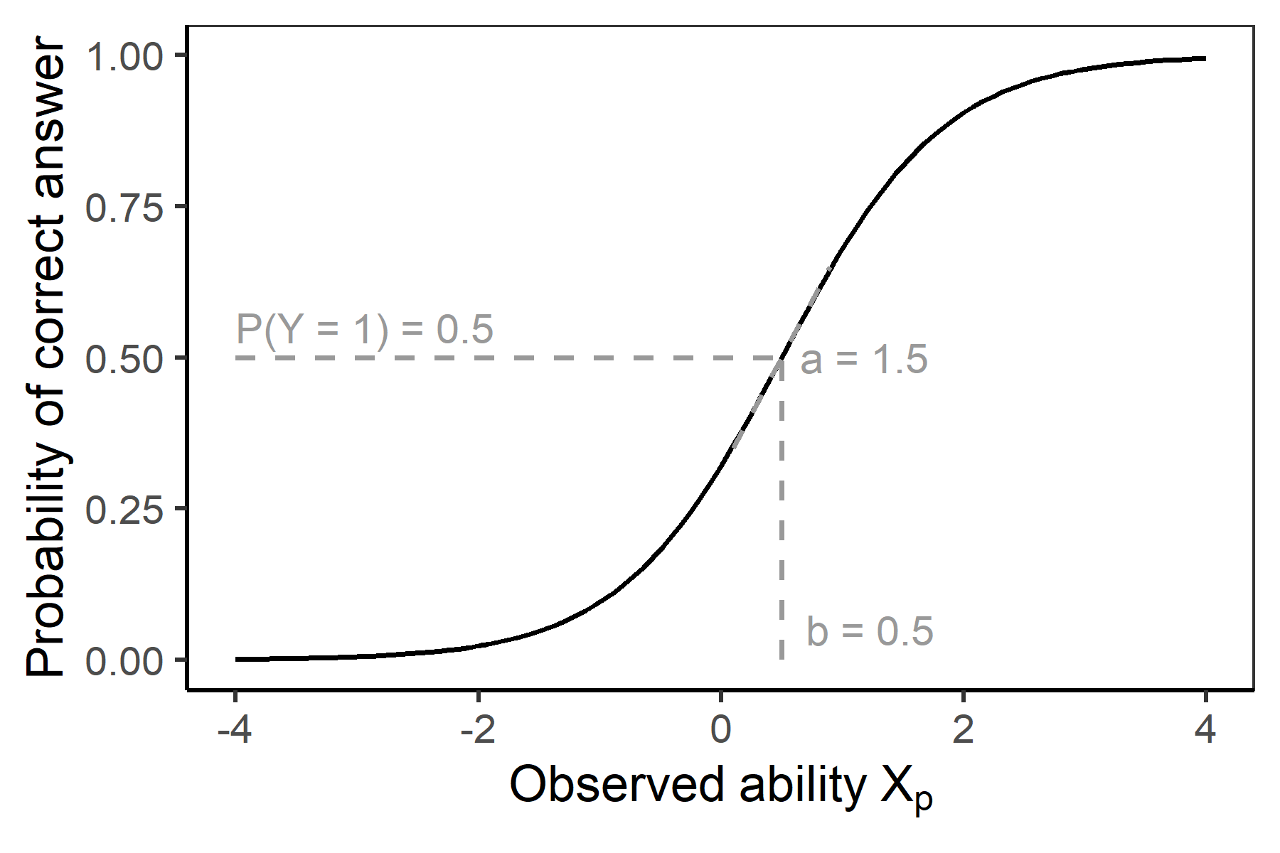
The relationship between the classical intercept-slope item parameters and the difficulty/discrimination parameters in the IRT parametrization is
\[ \begin{split} a_i &= \beta_{i1},\\ b_i &= -\frac{\beta_{i0}}{\beta_{i1}}. \end{split} \tag{6.9}\]
With transformation of the parameters, the standard errors will change as well. Standard errors of the new parameters can be obtained using the so-called delta method (see, for example, Doob, 1935). In the case where \(\widehat{\boldsymbol{\xi}}_i\) is a set of consistent estimates of item parameters \(\boldsymbol{\xi}_i\) with the asymptotic variance/covariance matrix \(\mathbb{\Sigma}_i\), then the asymptotic variance of the transformed estimates through function \(h\) is given by
\[ \nabla h(\boldsymbol{\xi}_i)^\top \mathbb{\Sigma}_i \nabla h(\boldsymbol{\xi}_i), \tag{6.10}\]
where \(\nabla h(\boldsymbol{\xi}_i)\) is a gradient of function \(h\), i.e., a vector of its partial derivatives with respect to parameters \(\boldsymbol{\xi}_i\).
IRT parametrization in R. Below, the estimated parameters for item 13 of the HCI dataset are transformed to IRT parametrization using Equation 6.9.
IRTpars13 <- c(coef(fit_2PL)[2], -coef(fit_2PL)[1] / coef(fit_2PL)[2])
setNames(IRTpars13, c("a", "b"))
a b
1.1824314 -0.4695603 The item difficulty is estimated at \(-0.47\) and the item discrimination is estimated at \(1.18\).
To enumerate the standard errors of the new parameters, the delta method may be implemented by hand by directly using the formula Equation 6.10 and the function deriv() of the base R to calculate the gradient \(h(\boldsymbol{\xi}_i)\) (see Supplementary R code for details). Here, the standard errors of the parameters are enumerated using the deltamethod() function from the msm package. It is necessary to specify function \(h\) through the argument g and original item estimates together with the estimated variance/covariance matrix.
library(msm)
deltamethod(g = list(~ x2, ~ -x1 / x2), mean = coef(fit_2PL), cov = vcov(fit_2PL))
[1] 0.10836769 0.08225591By interpreting the parameters for item 13 of the HCI dataset, we can say that a respondent with a total score \(0.47\) standard deviations below average (SE = \(0.08\)) has a probability of \(0.5\) to answer the item correctly. Interpretation (and value) of parameter \(a_i\) is the same as in the classical parametrization: With each standard deviation, the log-odds of answering the item correctly increases by the ratio of \(1.18\) (SE = 0.11).
The logistic regression model Equation 6.8 can be further generalized to account for the possibility that the answer to an item could be guessed correctly without possessing requisite knowledge, or that the item may be answered incorrectly by respondents of high ability due to inattention. Similarly, in psychological assessment, one may be interested in modeling the fact that some respondents do not endorse an item asking a culturally sensitive aspect of the tested trait. An example of such behavior is when a respondent with a high level of depression does not admit crying because they consider it socially or culturally unacceptable.
To account for the possibility of guessing, a non-zero lower asymptote \(c_i\) is added into the model. Such extension yields a 3PL model which no longer belongs to the GLM class of models. In the IRT parametrization, the model is defined as follows:
\[ \pi_{pi} = c_i + (1 - c_i)\frac{\exp(a_i(X_p - b_i))}{1 + \exp(a_i(X_p - b_i))}. \tag{6.11}\]
The new parameter \(c_i\) is called a guessing parameter, referring to guessing in multiple-choice items, or the pseudo-guessing parameter, admitting that processes other than just random guessing take place when a respondent selects between a number of offered options.
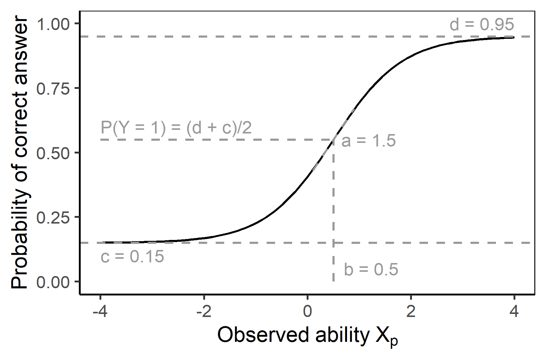
Interpretation of the difficulty parameter \(b_i\) now corresponds to the ability for which the respondent has the probability of a correct answer equal to \(\frac{1 + c_i}{2}\). Discrimination parameter \(a_i\) is related to the slope of the curve in this inflection point, with a slight change in the relationship: \(a_i\) is now the multiple of \(\frac{4}{1 - c_i}\) of the tangent of the angle at the inflection point. This can again be shown by taking a derivative of the probability function and by evaluating it at the inflection point \(b_i\):
\[ \left.\frac{\partial \pi_{pi}}{\partial X_p}\right\vert_{X_p = b_i} = \frac{(1 - c_i) a_i \exp (0)}{\left[1 + \exp (0)\right]^2} = \frac{a_i(1 - c_i)}{4}. \]
The 3PL model Equation 6.11 may be further extended by introducing the upper asymptote \(d_i\), also called the slipping parameter, the inattention parameter, or the lapse rate, which is possibly lower than 1, to account for a probability that the item was incorrectly answered despite the high ability \(X_p\). This yields a 4PL model:
\[ \pi_{pi} = c_i + (d_i - c_i)\frac{\exp(a_i(X_p - b_i))}{1 + \exp(a_i(X_p - b_i))}. \tag{6.12}\]
Interpretation of the parameters in the 4PL model is analogous to the one in the 3PL model. The guessing parameter \(c_i\) refers to the lower asymptote, i.e., the probability of answering the item correctly by a respondent with very low ability. The new parameter \(d_i\) corresponds to the upper asymptote, i.e., \(1-\) probability of answering the item incorrectly by a respondent with very high ability. The difficulty parameter \(b_i\) is again the location of an inflection point, when the respondent now has the probability of \(\frac{d_i + c_i}{2}\) of answering the item correctly. The slope parameter is now the multiple of \(\frac{a_i(d_i - c_i)}{4}\) of the tangent at the inflection point \(b_i\). For graphical illustration, see Figure 6.4.
Parameters in the nonlinear model Equation 6.11 can be estimated using several methods including the nonlinear least squares or the ML methods (see Section 6.5 for more information on parameter estimation).
3PL model in R. Here we show an estimation using the nonlinear least squares technique provided by the nls() function. We first define the formula of the 3PL nonlinear model to be fitted on the data:
mod_3PL <- function(x, a, b, c){
  c + (1 - c) * exp(a * (x - b)) /  (1 + exp(a * (x - b)))
}
The nls() function is then applied to fit the 3PL model Equation 6.11 on the data, while further specifying some other function arguments: To keep the parameter \(c_i\) within the limits of 0 and 1, the Port’s algorithm is used with further arguments lower and upper for the limits. We also need to specify initial values since this is not done automatically, as was the case for the glm() function. Quality of the starting values may influence the convergence of the algorithm. A possible choice is to use the traditional item analysis parameters as the starting values. Here we choose fixed starting values for illustration purposes. We once again demonstrate fitting the 3PL model on item 13 of the HCI dataset.
fit_3PL <- nls(HCI[, 13] ~ mod_3PL(zscore, a, b, c),
               algorithm = "port", start = c(a = 0.7, b = -0.9, c = 0),
               lower = c(-Inf, -Inf, 0), upper = c(Inf, Inf, 1))
We print the estimated model parameters and their standard errors:
coef(fit_3PL) a b c
2.6691902 0.2707837 0.3214444 sqrt(diag(vcov(fit_3PL))) a b c
0.52763750 0.09075821 0.03934340 Interpreting the estimated guessing parameter \(c_i\), respondents would have \(0.32\) (SE = 0.53) probability of answering item 13 correctly even in a case where their ability was very low. Parameter \(b_i = 0.27\) (SE = 0.09) now corresponds to the respondents’ observed ability (Z-score) for which the probability of correctly answering item 13 is in the middle between guessing and 1, i.e., \(\frac{1 + 0.32}{2} = 0.66\) (see also Figure 6.5).
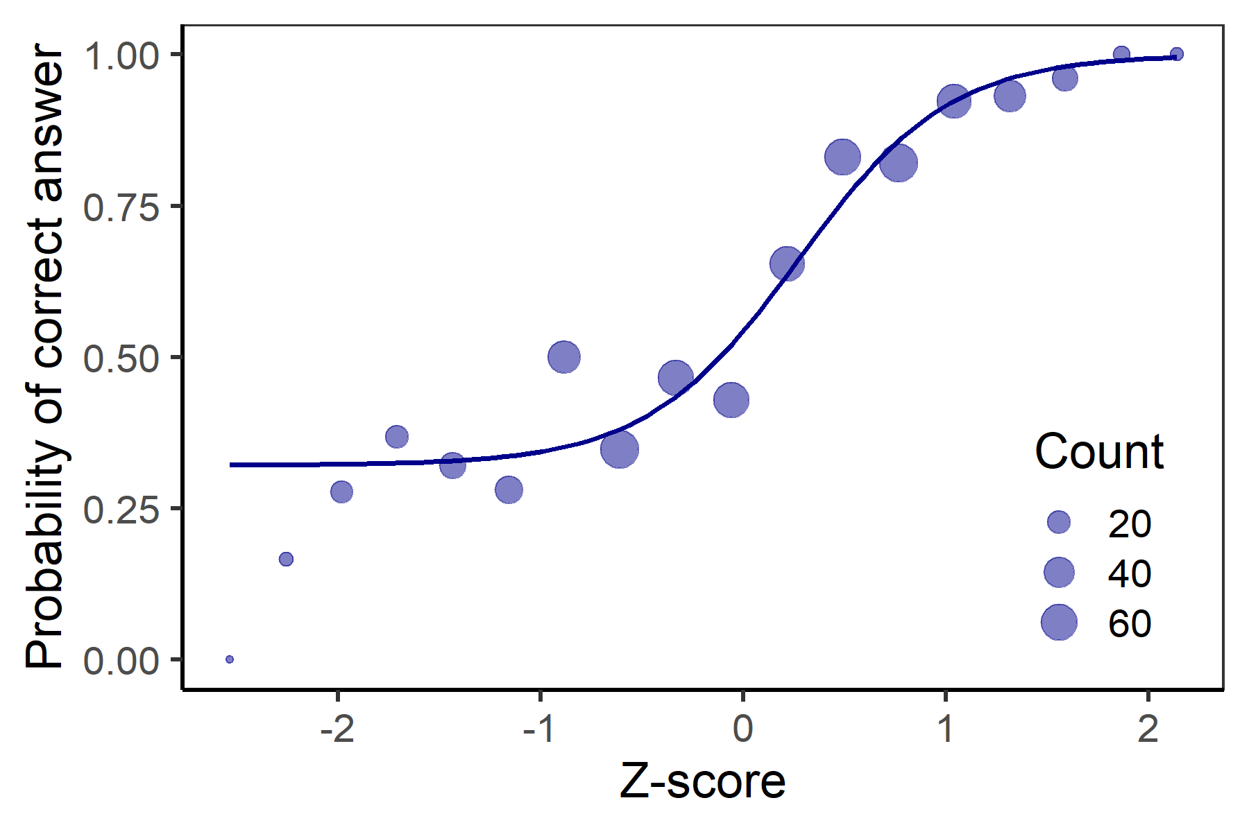
HCI dataset.
4PL model in R. To model the functioning of an item with the 4PL nonlinear model Equation 6.12, we first define the nonlinear function
mod_4PL <- function(x, a, b, c, d){
  c + (d - c) * exp(a * (x - b)) / (1 + exp(a * (x - b)))
}
We then fit the model on item 13 of the HCI dataset with the nls() function as we did with the 3PL model above. The lower limits for the last two parameters c and d are set at 0 and their upper limits are set at 1.
fit_4PL <- nls(HCI[, 13] ~ mod_4PL(zscore, a, b, c, d),
               algorithm = "port", start = c(a = 0.7, b = -0.9, c = 0, d = 1),
               lower = c(-Inf, -Inf, 0, 0), upper = c(Inf, Inf, 1, 1))
The model parameters and their standard errors are again printed using the coef() and the vcov() functions.
coef(fit_4PL) a b c d
3.3404997 0.2325763 0.3379216 0.9569426 sqrt(diag(vcov(fit_4PL))) a b c d
0.98459974 0.09919667 0.03626136 0.04998790 In item 13 of the HCI data, the inattention parameter is estimated to be 0.96 (SE = 0.05), and the model is very similar to the 3PL model fit_3PL estimated above.
In this section, we present extensions of the two main approaches for the parameter estimation presented in Section 4.3: Those based on minimization of the RSS and those based on ML; see also Hladká et al. (2023) for discussion.
The nonlinear least squares method is based on minimization of the RSS. In case of the 2PL model Equation 6.8, the RSS for item \(i\) has the form:
\[ \text{RSS}_i = \sum_{p = 1}^{n} \left(Y_{pi} - \pi_{pi}\right)^2 = \sum_{p = 1}^{n} \left(Y_{pi} - \frac{\exp\left(a_i(X_p - b_i)\right)}{1 + \exp\left(a_i(X_p - b_i)\right)} \right)^2. \]
This leads to a system of two nonlinear estimating equations \(\frac{\partial \text{RSS}_i}{\partial a_i} = 0,\) \(\frac{\partial \text{RSS}_i}{\partial b_i} = 0.\) Unlike in the linear regression model, no explicit formulae are available, and numerical approaches need to be applied to solve the equations.
In the case of the nonlinear 4PL model Equation 6.12, the RSS has the form:
\[ \text{RSS}_i = \sum_{p = 1}^{n} \left[Y_{pi} - \pi_{pi}\right]^2 = \sum_{p = 1}^{n} \left[Y_{pi} - c_i - (d_i - c_i) \frac{\exp\left(a_i(X_p - b_i)\right)}{1 + \exp\left(a_i(X_p - b_i)\right)} \right]^2, \]
which leads to a system of four nonlinear estimating equations \(\frac{\partial \text{RSS}_i}{\partial a_i} = 0,\) \(\frac{\partial \text{RSS}_i}{\partial b_i} = 0,\) \(\frac{\partial \text{RSS}_i}{\partial c_i} = 0,\) \(\frac{\partial \text{RSS}_i}{\partial d_i} = 0,\) with constraints on parameters \(c_i\) and \(d_i\). Again, no explicit formulae are available, and numerical approaches are needed; for example, the “nl2sol” algorithm from the Port library (Dennis et al., 1981; Gay, n.d.) may be used.
For GLM such as logistic or probit regression, the ML method is typically used for parameter estimation. The likelihood function for the item \(i\) enumerates the probability of response vector \(\boldsymbol{Y}_i\) taking a vector of values \(\boldsymbol{y}_{i}\) given the item parameters \(\boldsymbol{\xi}_i\). For binary items \(Y_{pi}\) with \(\pi_{pi}\) defined by the 2PL model Equation 6.4, the 3PL model Equation 6.11, or the 4PL model Equation 6.12, and under the assumption that the respondent’s answers are independent, it takes the form:
\[ L_i(\boldsymbol{\xi}_i) = \prod_{p = 1}^n \text{P}(\boldsymbol{Y}_{i} = \boldsymbol{y}_{i}| \boldsymbol{\xi}_i) = \prod_{p = 1}^n \pi_{pi}^{y_{pi}} \left(1 - \pi_{pi}\right)^{1 - y_{pi}}. \tag{6.13}\]
The log-likelihood function for the item \(i\) is then given by
\[ l_{i}(\boldsymbol{\xi}_i) = \sum_{p = 1}^n \left[y_{pi} \log(\pi_{pi}) + (1 - y_{pi})\log(1 - \pi_{pi})\right]. \tag{6.14}\]
Parameter estimation involves the maximization of \(l_i(\boldsymbol{\xi}_i)\) with respect to item parameters \(\boldsymbol{\xi}_i\) which leads to a system of likelihood equations of the same number as the number of the model parameters; for the 4PL model \(\frac{\partial l_i(\boldsymbol{\xi}_i)}{\partial a_i} = 0,\) \(\frac{\partial l_i(\boldsymbol{\xi}_i)}{\partial b_i} = 0,\) \(\frac{\partial l_i(\boldsymbol{\xi}_i)}{\partial c_i} = 0,\) \(\frac{\partial l_i(\boldsymbol{\xi}_i)}{\partial d_i} = 0,\) with constraints on parameters \(c_i\) and \(d_i.\) No solution of a closed form is available, and numerical algorithms are needed. For the 2PL model, this leads to an IRLS algorithm. For the 3PL and 4PL model, the modification of the quasi-Newton method may be used, allowing for box constraints (Byrd et al., 1995).
An important task in the description of item functioning is deciding about how many parameters are needed. For example, we may want to test a hypothesis that the discrimination parameter is equal to some constant (presumably the same constant for all items), or we might be interested in whether a nonzero guessing parameter needs to be considered in the model.
The LRT Equation 2.29 discussed in Chapter 2 might be used to compare model \(M_{iH_1}\) for item \(i\) and its submodel \(M_{iH_0}\). Note, however, that for testing the 2PL versus the 3PL or 4PL model, the LRT is not suitable, because the parameters \(c_i\) and \(d_i\) are bounded by interval \([0, 1]\), and boundary values violate asymptotic properties of the test.
The AIC Equation 2.30 may be used to assess the goodness of fit by
\[ \mathrm{AIC} = 2k - 2 \log(L_i(\hat{\boldsymbol{\xi}}_i)) \tag{6.15}\]
with \(L_i(\hat{\boldsymbol{\xi}}_i)\) being the maximized likelihood function for item \(i\), and \(k\) being the number of estimated parameters used as a penalty. Recall that when comparing multiple models, the model with the lowest AIC value is the preferred one.
Akaike information criterion in R. In R, the AIC() function may be used to extract AIC Equation 6.15 from several objects including those returned by the glm() or nls() functions. However, the compared models should be fitted using the same method.
Here we compare the 3PL and 4PL models for item 13 of the HCI dataset, previously fitted with the nls() function.
AIC(fit_3PL, fit_4PL) df AIC
fit_3PL 4 740.8746
fit_4PL 5 742.4880According to the AIC, the 3PL model shows a better fit, whereas the AIC is lower.
The BIC Equation 2.31 may be used to assess goodness of model fit while more strictly penalizing the number of parameters:
\[ \mathrm{BIC} = k \log(n) - 2 \log(L_i(\hat{\boldsymbol{\xi}}_i)). \tag{6.16}\]
Once again, lower values of the BIC signalize a better fitting model.
Bayesian information criterion in R. The BIC() function might be used to extract BIC Equation 6.16 for the 3PL and 4PL models for item 13 of the HCI.
BIC(fit_3PL, fit_4PL) df BIC
fit_3PL 4 758.7886
fit_4PL 5 764.8806According to BIC, the 3PL model fit_3PL is once more preferred over the 4PL model, whereas the BIC is lower.
Polytomous items are often present in educational, psychological, and health-related measurements. Examples include partial credit ordinal items, Likert-type ordinal items asking the respondents to rate offered statements on a scale such as “Strongly disagree”–“Disagree”–“Agree”–“Strongly agree”, or the multiple-choice nominal item asking the respondents to select the best answer.
As was shown in Examples for Chapter 1, with ordinal items it is possible to dichotomize the data by cut-point, e.g., by assigning 1 to a fully correct answer and 0 otherwise, or to assign 1 to “Agree” and “Strongly agree” options and 0 otherwise. However, this may discard valuable information about the ability level needed to move from one category (e.g., zero points) to another (e.g., partial credit) or the trait level needed to “Strongly agree” on the offered statement.
Similarly, in multiple-choice items, dichotomization of the data, i.e., analyzing the correct answer only, may lead to discarding valuable information on the functioning of incorrect options (distractors), which may be key for diagnosis and the further treatment of misconceptions. Models for polytomous items – ordinal and nominal regression models – make full use of the data.
Ordinal regression allows for modeling Likert-scale and partial-credit items. The models differ in how they employ the link function, either for cumulative probabilities or for the probabilities of adjacent categories. The results are typically similar; the choice should depend on the usage: For Likert scale items, the cumulative logit model may be more appropriate. For partial credit items, one may consider an adjacent-categories logit model which can better describe the ability needed to transition from partial mastery to a more complete one.
The cumulative logit models are appropriate for modeling ordinal items especially in cases where the main interest is in the probabilities of gaining at least a certain cut-score \(k\). Considering \(K_i + 1\) ordered categories of item \(i\), \(k = 0, \dots, K_i\), the cumulative probability of getting at least \(k\) points is modeled using the logistic regression Equation 6.4:
\[ \pi^{*}_{pik} \coloneqq \text{P}(Y_{pi} \geq k|X_p) = \frac{\exp\left(\beta_{i0k} + \beta_{i1}X_p\right)}{1 + \exp\left(\beta_{i0k} + \beta_{i1}X_p\right)} \quad k = 1, \dots, K_i, \tag{6.17}\]
while for the first category \(\pi^{*}_{pi0} = 1\), whereas there is no lower category. In this model, \(X_p\) is again an observed ability of the respondent \(p\). Parameters \(\beta_{i0k}\) describe category locations and parameter \(\beta_{i1}\) is a common slope for all categories within item \(i\). Because the cumulative probabilities are ordered, i.e., \(\pi^{*}_{pi0} \geq \pi^{*}_{pi1} \geq \dots \pi^{*}_{piK_i},\) the location parameters are also ordered, i.e., \(\beta_{i01} \geq \dots \geq \beta_{i0K_i}.\)
In other words, the cumulative logit model assumes a linear form for a logarithm of the odds of getting at least \(k\) points, i.e., for the cumulative logits:
\[ \text{logit}(\pi^{*}_{pik}) \coloneqq \log\left(\frac{\pi^{*}_{pik}}{1 - \pi^{*}_{pik}}\right) = \beta_{i0k} + \beta_{i1}X_p, \quad k = 1, \dots, K_i, \]
and the model thus belongs to the class of GLM.
Using the IRT parametrization, the cumulative probabilities are modeled as
\[ \pi^{*}_{pik} = \frac{\exp\left(a_i(X_p - b_{ik})\right)}{1 + \exp\left(a_i(X_p - b_{ik})\right)}, \quad k = 1, \dots, K_i, \tag{6.18}\]
where \(b_{i1} < b_{i2} < \dots b_{iK_i}\).
In this parametrization of the model, parameter \(a_{i}\) is a common slope for all categories within item \(i\), and parameters \(b_{ik}\) are locations of inflection points of cumulative probability functions, i.e., the abilities for which the probability of endorsing a given category or a higher one is exactly 50%.
The relationship between the parameters in intercept-slope parametrization Equation 6.17 and in the IRT parametrization Equation 6.18 for item \(i\) is analogous to Equation 6.9:
\[ \begin{split} a_i &= \beta_{i1},\\ b_{ik} &= -\frac{\beta_{i0k}}{\beta_{i1}}, \quad k = 1, \dots, K_i. \end{split} \tag{6.19}\]
Standard errors under the IRT parametrization can be obtained using the delta method Equation 6.10.
The response category probabilities are given by differences in cumulative probabilities, while the response category probability of the last category is equal to its cumulative probability, whereas there is no higher category:
\[ \begin{split} \pi_{pik} \coloneqq & \ \text{P}(Y_{pi} = k|X_p) = \pi^{*}_{pik} - \pi^{*}_{pi(k + 1)}, \quad k = 0, \dots, K_i - 1, \\ \pi_{piK_i} \coloneqq & \ \pi^{*}_{piK_i}. \end{split} \tag{6.20}\]
The sum of all category probabilities is equal to 1, as expected:
\[ \sum_{k = 0}^{K_i} \pi_{pik} = (\pi^{*}_{pi0} - \pi^{*}_{pi1}) + (\pi^{*}_{pi1} - \pi^{*}_{pi2}) + \dots + (\pi^{*}_{pi(K_i - 1)} - \pi^{*}_{piK_i}) + \pi^{*}_{piK_i} = \pi^{*}_{pi0} = 1. \]
When there are only two response categories 0 and 1, i.e., when \(K_i = 1\), the cumulative logit model Equation 6.18 reduces to the logistic regression model Equation 6.8.
Cumulative logit model in the VGAM package. To illustrate fitting and interpretation of the cumulative logit regression model, we will use the Anxiety dataset. It includes 29 Likert-type items asking the respondents to rate offered statements on a scale “Never” – “Rarely” – “Sometimes” – “Often” – “Always” coded as 1 to 5. We will use item 18 with the statement “I worried about other people’s reactions to me”. For more details, see Section 1.3. We first extract the Z-scores. We then recode the item responses to 0–4 and we use the ordered() function to create a factor variable with ordered values for item 18.
data("Anxiety", package = "ShinyItemAnalysis")
zscore <- Anxiety$zscore
Anxiety_items <- Anxiety[, paste0("R", 1:29)] - 1
Anxiety_items$R18 <- ordered(factor(Anxiety_items$R18,
                             levels = 0:max(Anxiety_items$R18)))
The vglm() function from the VGAM package is used with argument family = cumulative to fit the cumulative logit model Equation 6.17. Note that the argument reverse = TRUE is needed to obtain required model specification.
library(VGAM)Loading required package: stats4Loading required package: splinesfit_cum <- vglm(Anxiety_items$R18 ~ zscore,
family = cumulative(reverse = TRUE, parallel = TRUE))Model summary can be accessed with the summary() method (see Supplementary R code).
We use the coef() method to obtain estimated item parameters, while the standard errors are available from the diagonal of the variance/covariance matrix provided by the vcov() method. The vglm() function uses a classical intercept-slope parametrization Equation 6.17.
coef(fit_cum)(Intercept):1 (Intercept):2 (Intercept):3 (Intercept):4 zscore
0.4154705 -1.2806717 -3.4374075 -5.1977515 1.7324772 sqrt(diag(vcov(fit_cum)))(Intercept):1 (Intercept):2 (Intercept):3 (Intercept):4 zscore
0.08646028 0.10310049 0.18248212 0.28801644 0.09545942 Before interpreting the estimated item parameters, we use Equation 6.19 to obtain parameters using the IRT notation Equation 6.18.
c(-coef(fit_cum)[1:4] / coef(fit_cum)[5], coef(fit_cum)[5])(Intercept):1 (Intercept):2 (Intercept):3 (Intercept):4 zscore
-0.2398130 0.7392142 1.9840997 3.0001847 1.7324772 The delta method Equation 6.10 is implemented with the deltamethod() function from the msm package to obtain the standard errors of the item parameters under the IRT parametrization.
deltamethod(list(~ -x1 / x5, ~ -x2 / x5, ~ -x3 / x5, ~ -x4 / x5, ~ x5),
            mean = coef(fit_cum), cov = vcov(fit_cum))
[1] 0.04863660 0.06434982 0.10331593 0.16099682 0.09545942From the estimated model, it follows that a respondent with Z-score of \(-0.24\) (SE = 0.05); i.e., with an observed level of anxiety slightly below average, has 50% probability of answering at least “Rarely”; a respondent with Z-score of \(0.74\) (SE = 0.06), i.e., with a level of anxiety somewhat above average, has 50% probability of answering at least “Sometimes”, etc. With each unit increase of the Z-score, the log-odds of endorsing a given category, or a higher one, increases by the ratio of \(1.73\) (SE = 0.10).
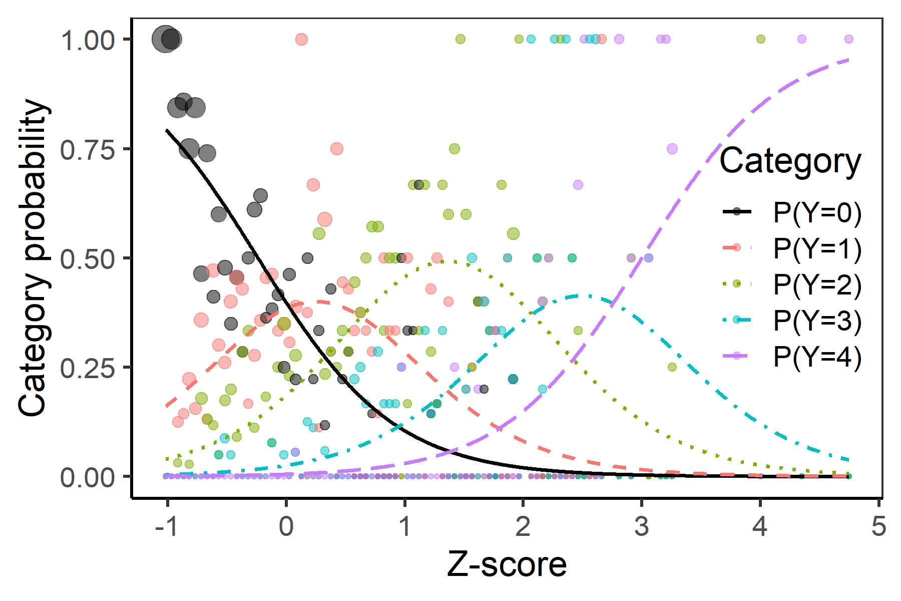
Cumulative probabilities are plotted using the plotCumulative() function from the ShinyItemAnalysis package with argument type = "cumulative". Argument type = "category" is used to plot the category probabilities. See Supplementary R code for further plotting options to produce the figures.
library(ShinyItemAnalysis)This is ShinyItemAnalysis version 1.5.5
- to run the interactive {shiny} app, call `run_app()`
- to learn more, visit `ShinyItemAnalysis.org`
Attaching package: 'ShinyItemAnalysis'The following object is masked _by_ '.GlobalEnv':
EPIAplotCumulative(fit_cum, type = "cumulative")Warning: Using `size` aesthetic for lines was deprecated in ggplot2 3.4.0.
ℹ Please use `linewidth` instead.
ℹ The deprecated feature was likely used in the ShinyItemAnalysis package.
Please report the issue at
<https://github.com/patriciamar/ShinyItemAnalysis/issues>.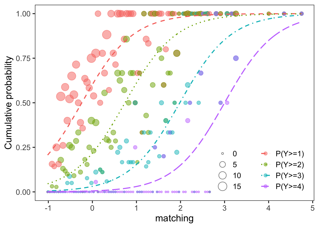
plotCumulative(fit_cum, type = "category")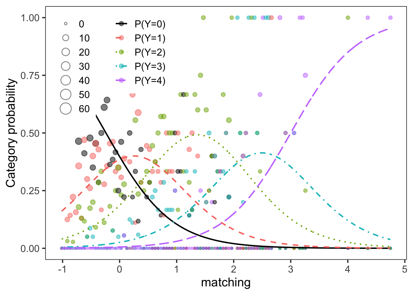
knitr::include_graphics("figures/regression_cumulative_Anxiety_cumulative_item18.png")
knitr::include_graphics("figures/regression_cumulative_Anxiety_category_item18.png")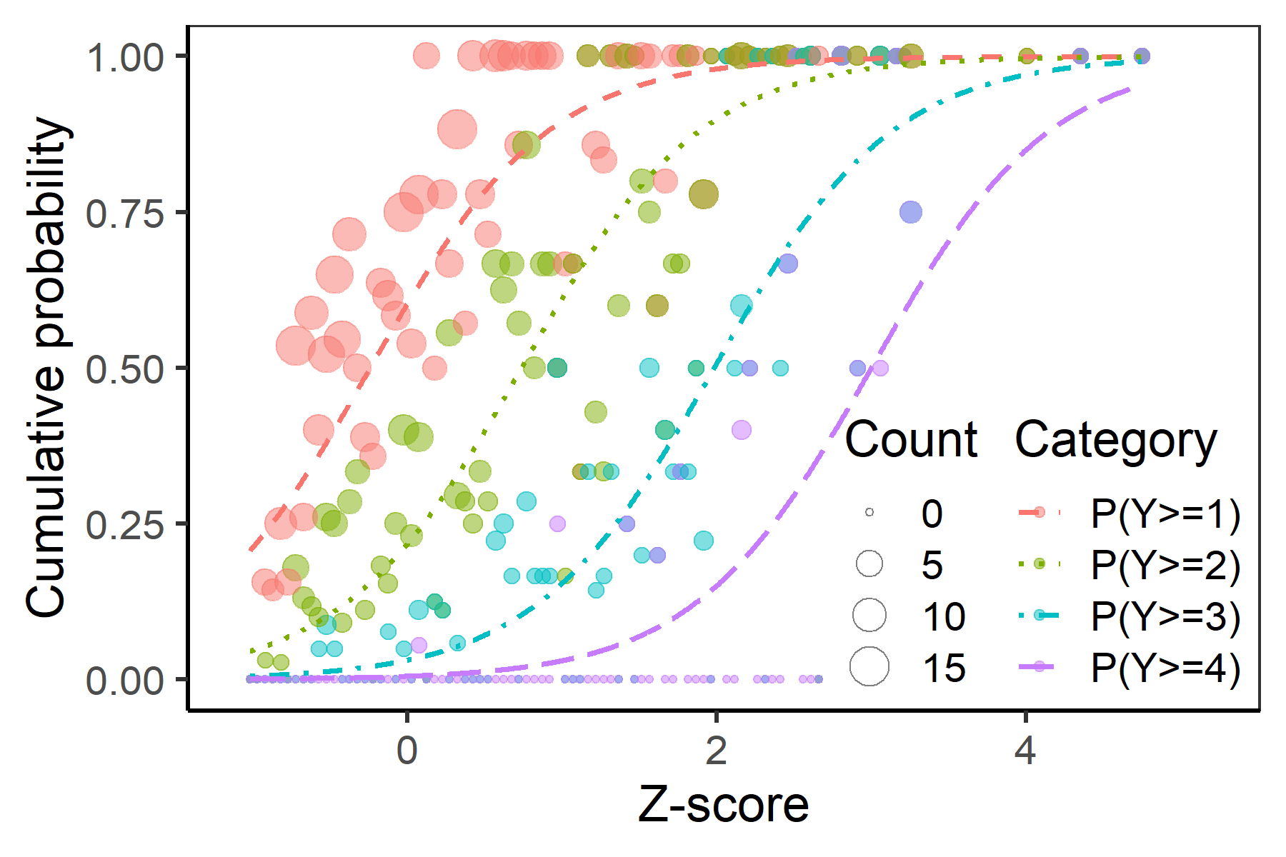
Anxiety dataset.
The estimated item parameters can be read from the plot of cumulative probabilities (Figure 9.8 (a)) as locations of inflection points and slopes of the curves at these inflection points. The category probability plot (Figure 9.8 (b)) displays probabilities of each category given the observed ability (Z-score). Note that for each Z-score, the probabilities for all categories add up to 1.
The adjacent-categories logit model is useful for describing functioning of ordinal items when the interest is in the level of ability needed to move from one category to the next one. Considering an ordinal item \(i\) with \(K_i + 1\) categories \(k = 0, \dots, K_i,\) the model assumes a linear form of logarithm for the ratio of probabilities for two successive scores (e.g., 0 vs. 1, 1 vs. 2, 2 vs. 3, etc.), the so-called adjacent-categories logits. In the intercept-slope parametrization, the model is specified as
\[ \log\left(\frac{\pi_{pik}}{\pi_{pi(k - 1)}}\right) = \beta_{i0k} + \beta_{i1}X_p, \quad k = 1, \dots, K_i, \tag{6.21}\]
where \(\beta_{i0k}\) are category-specific intercept parameters, and \(\beta_{i1}\) is a common slope parameter for item \(i\). The model thus belongs to the class of GLM.
In the IRT parametrization, the model is specified as
\[ \log\left(\frac{\pi_{pik}}{\pi_{pi(k - 1)}}\right) = a_{i}(X_p - b_{ik}), \quad k = 1, \dots, K_i. \tag{6.22}\]
In this parametrization, \(a_i\) is once more the common slope. Parameters \(b_{ik}\) have a nice graphical interpretation: They are the threshold parameters corresponding to observed ability for which the adjacent categories intersect. This can be observed from Equation 6.22: When \(X_p = b_{ik}\), then the adjacent-categories probabilities are equal \(\pi_{pik} = \pi_{pi(k - 1)}\). In other words, \(b_{ik}\) corresponds to the observed ability required to transition from category \(k - 1\) to the next category \(k\).
The relationship between the parameters in Equation 6.21 and Equation 6.22 is as in Equation 6.19. The standard errors in the IRT parametrization can be calculated from those in the intercept-slope parametrization using the delta method Equation 6.10.
In the IRT parametrization, the response category probabilities can be derived from Equation 6.22 using a recursive formula, and they take the form:
\[ \begin{split} \pi_{pik} &= \frac{\exp\left(\sum_{l = 1}^{k} a_i (X_p - b_{il})\right)}{1 + \sum_{t = 1}^{K_i} \exp\left(\sum_{l = 1}^t a_i (X_p - b_{il})\right)}, \quad k = 1, \dots, K_i,\\ \pi_{pi0} &= \frac{1}{1 + \sum_{t = 1}^{K_i} \exp\left(\sum_{l = 1}^t a_i (X_p - b_{il})\right)} = 1 - \sum_{k = 1}^{K_i} \pi_{pik}. \end{split} \tag{6.23}\]
When there are only two response categories 0 and 1, i.e., when \(K_i = 1\), the adjacent-categories logit model Equation 9.14 reduces to the logistic regression model Equation 6.8.
Adjacent-categories logit model in the VGAM package. We again demonstrate the fitting of the model on the Anxiety dataset and its item 18. The adjacent-categories logit model Equation 6.21 is fitted via the vglm() function from the VGAM package using the argument family = acat(reverse = FALSE, parallel = TRUE).
fit_adj <- vglm(Anxiety_items$R18 ~ zscore,
                family = acat(reverse = FALSE, parallel = TRUE))
Estimated parameters and standard errors in the intercept-slope parametrization Equation 6.21 are again computed with the coef() and vcov() methods.
coef(fit_adj)(Intercept):1 (Intercept):2 (Intercept):3 (Intercept):4 zscore
-0.2321577 -0.5296378 -2.2145620 -2.7409576 1.0109268 sqrt(diag(vcov(fit_adj)))(Intercept):1 (Intercept):2 (Intercept):3 (Intercept):4 zscore
0.09759614 0.11826503 0.21106258 0.33474901 0.07215644 Before providing interpretation, we use transformation Equation 6.19 to obtain parameters under the IRT parametrization Equation 6.22. The standard errors of the new parameters are computed using the delta method Equation 6.10 with the deltamethod() function from the msm package.
c(-coef(fit_adj)[1:4] / coef(fit_adj)[5], coef(fit_adj)[5])(Intercept):1 (Intercept):2 (Intercept):3 (Intercept):4 zscore
0.2296484 0.5239131 2.1906255 2.7113314 1.0109268 deltamethod(list(~ -x1 / x5, ~ -x2 / x5, ~ -x3 / x5, ~ -x4 / x5, ~ x5),
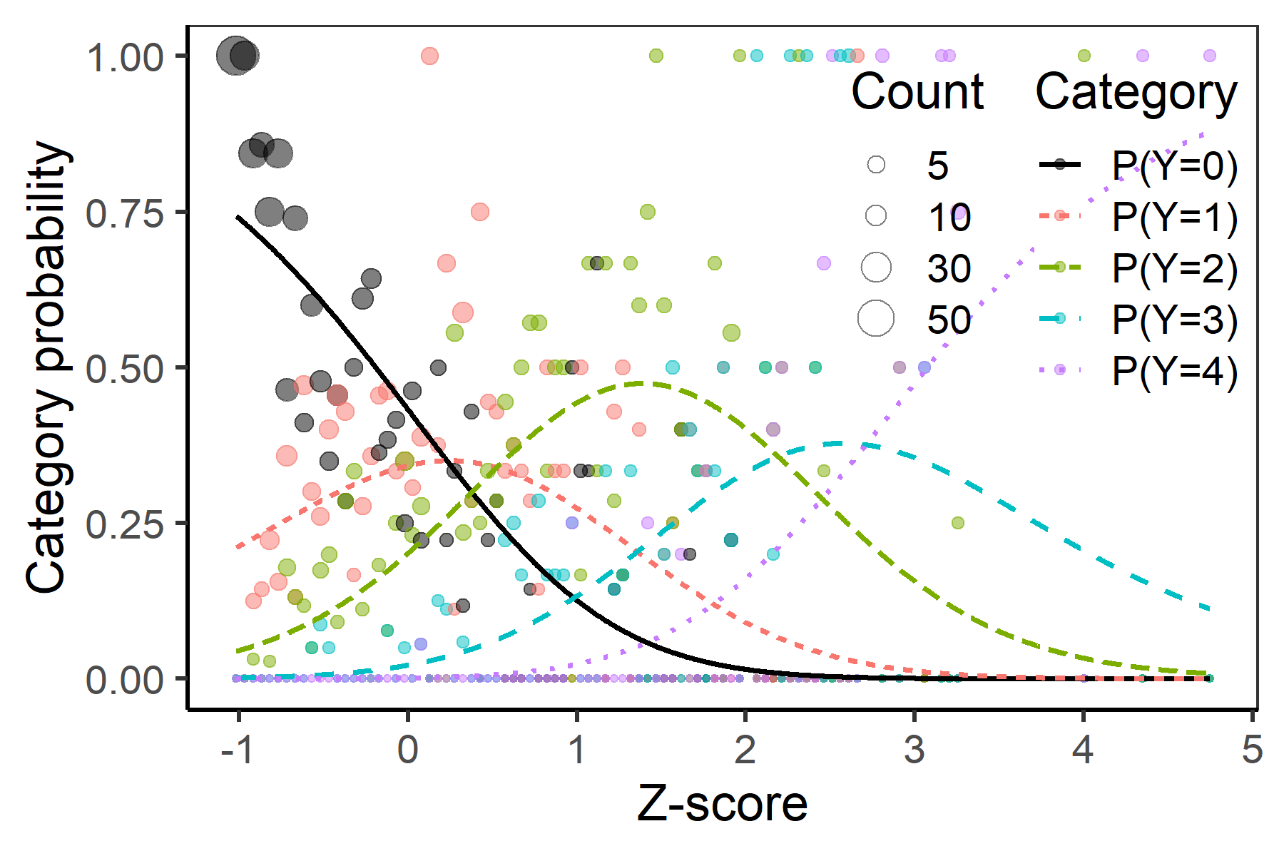
mean = coef(fit_adj), cov = vcov(fit_adj))[1] 0.10348436 0.11629492 0.18736261 0.27692177 0.07215644Estimated parameters can be interpreted as follows: A respondent with a Z-score of \(0.23\) (anxiety level 0.23 SD above average, SE = 0.10) has equal probability to endorse the option “Rarely” and “Never” in item 18; in other words, a Z-score of \(0.23\) is needed to transition between these two categories. Similarly, a Z-score of \(0.52\) (SE = 0.12) is needed to transition between the option “Sometimes” and “Rarely”, etc.
Estimated category probabilities can be plotted with the plotAdjacent() function from the ShinyItemAnalysis package.
plotAdjacent(fit_adj, matching.name = "Z-score")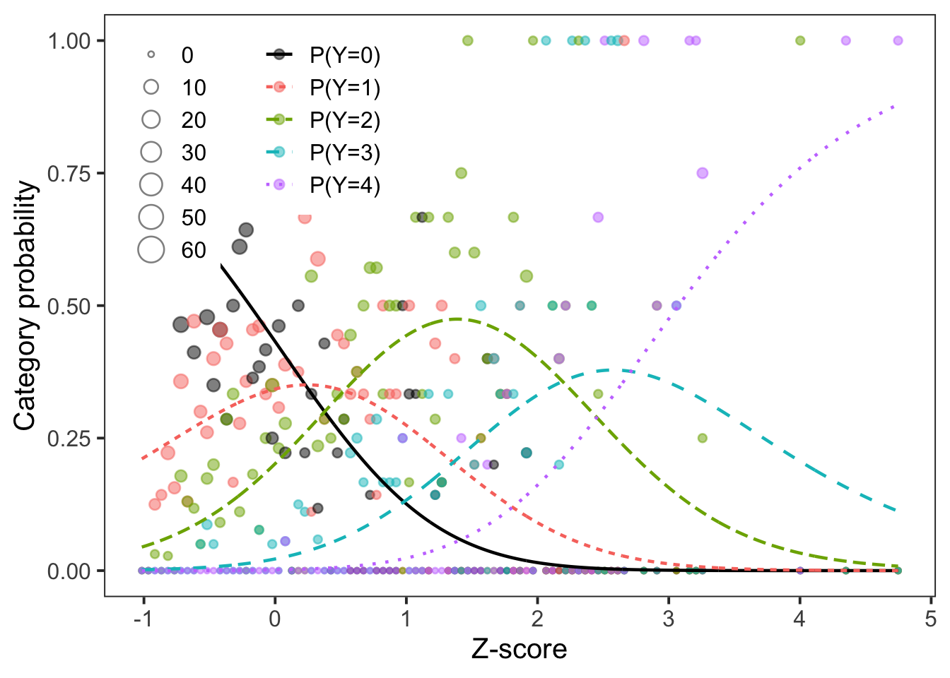
Anxiety dataset.
The locations of the intersections of adjacent category probability curves correspond to the “Intercept” parameter estimates \(b_{ik}\) using the IRT parametrization (Figure 9.9).
Multinomial regression can be used to model responses for all given options (i.e., the correct response and all distractors), in multiple-choice items. For item \(i\) with \(K_i\) categories and \(k = 0\) being the index of the baseline category, the multinomial regression model, also called the baseline-category logit model, assumes linear form in the log-odds of choosing option \(k \neq 0\) vs. the baseline category \(k = 0\) when restricting the data to these two options. In the intercept-slope parametrization, the model is defined as:
\[ \log\left(\frac{\pi_{pik}}{\pi_{ip0}}\right) = \beta_{0ik} + \beta_{1ik}X_p, \quad k = 1, \dots, K_i, \tag{6.24}\]
with category-specific intercept parameters \(\beta_{0ik}\) and category-specific slope parameters \(\beta_{1ik}.\)
In the IRT parametrization the model is defined by a set of equations:
\[ \log\left(\frac{\pi_{pik}}{\pi_{ip0}}\right) = a_{ik}(X_p - b_{ik}), \quad k = 1, \dots, K_i, \tag{6.25}\]
with category-specific slopes \(a_{ik}\), and category-specific difficulty parameters \(b_{ik}\) which can be interpreted as the observed ability levels needed to transition from category \(k \neq 0\) to the baseline category \(k = 0.\) As can be read from Equation 6.25, for observed ability \(X_p = b_{ik},\) the probability \(\pi_{pik}\) of response option \(k\) is equal to the probability \(\pi_{pi0}\) of the baseline response category \(0\).
The relationship between the two sets of parameters is similar to Equation 6.19, namely
\[ \begin{split} a_{ik} &= \beta_{i1k},\\ b_{ik} &= -\frac{\beta_{i0k}}{\beta_{i1}}, \quad k = 1, \dots, K_i. \end{split} \tag{6.26}\]
The standard errors of parameters \(a_{ik}\) and \(b_{ik}\) in the IRT parametrization Equation 6.25 can be calculated from a variance/covariance matrix of the parameters in the intercept-slope parametrization Equation 6.24 using Equation 6.26 and the delta method Equation 6.10.
Response category probabilities then take the form of the ratio between category-related functions and their sum, while the probability of the baseline category is calculated from the remaining response categories:
\[ \begin{split} \pi_{pik} &= \frac{\exp\left(a_{ik}(X_p - b_{ik})\right)}{1 + \sum_{l = 1}^{K_i}\exp\left(a_{il}(X_p - b_{il})\right)},\\ \pi_{pi0} &= \frac{1}{1 + \sum_{l = 1}^{K_i}\exp\left(a_{il}(X_p - b_{il})\right)} = 1 - \sum_{k = 1}^{K_i} \pi_{pik}; \end{split} \tag{6.27}\]
The multinomial regression model Equation 6.25 is a generalization of the adjacent-categories logit model Equation 6.22 in that it allows different slope parameters \(a_{ik}\) for each item category. In order to define the same model, the slope parameters \(a_{ik}\) in the multinomial model have to be set to multiples of the slope parameter (here denoted \(\tilde{a}_{i}\)) in the adjacent-categories logit model. In the adjacent-categories logit model, the location parameters (here denoted \(\tilde{b}_{ik}\)) are the locations of intersections between adjacent categories (Figure 6.8 (a)), while in the multinomial model, parameters \(b_{ik}\) are locations of response probability curves intersections with the baseline category (Figure 6.8 (b)).
knitr::include_graphics("figures/regression_illustrative_ACLM_vs_BCLM_ACLM.png")
knitr::include_graphics("figures/regression_illustrative_ACLM_vs_BCLM_BCLM.png")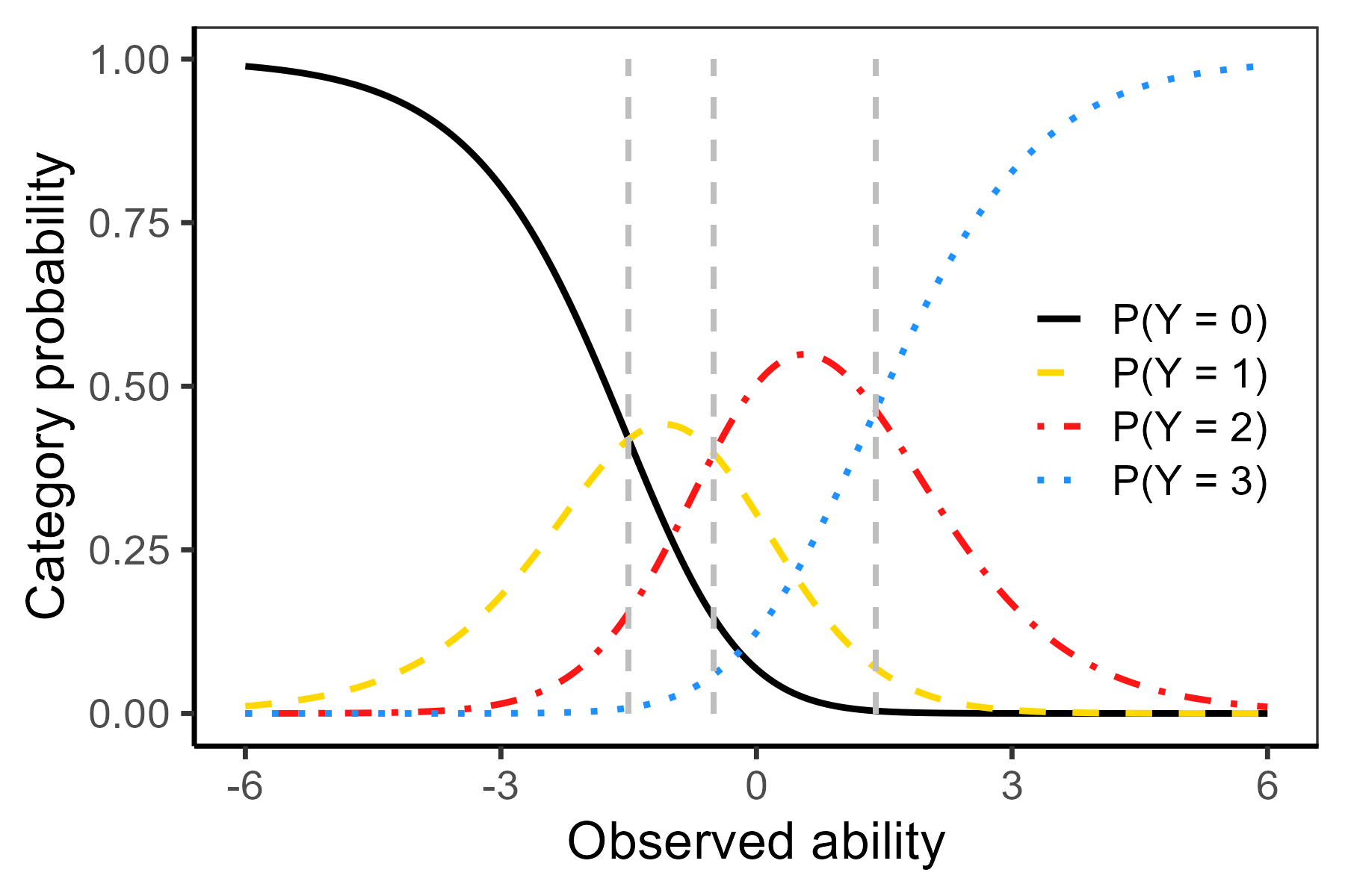
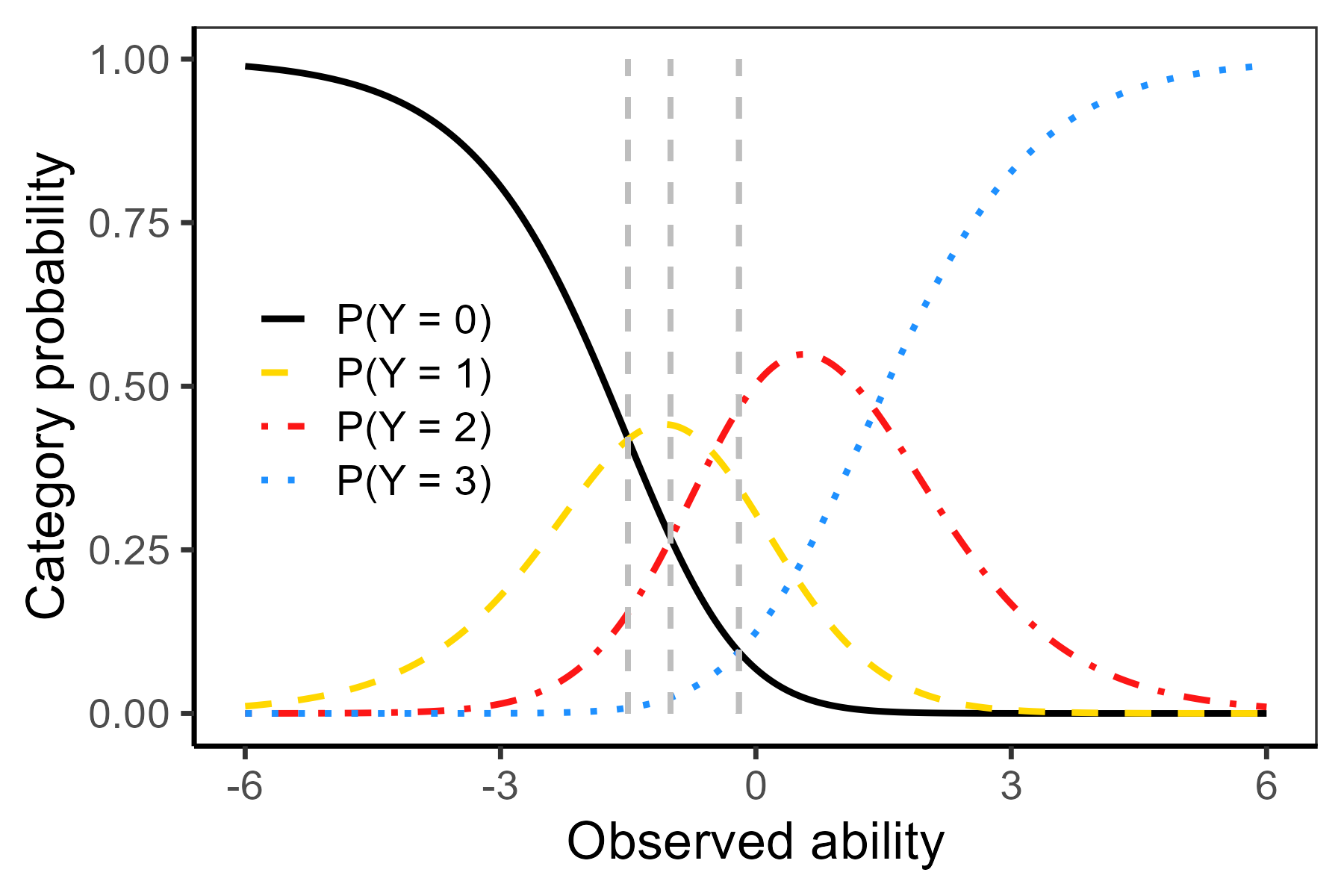
The relationship between the two sets of parameters is derived from setting the response category probabilities in the adjacent-categories logit model Equation 9.14 and in the baseline-category logit model Equation 6.27 equal, and thus by setting the nominators of the two expressions equal for each category \(k = 1, \dots, K_i\). An illustrative recalculation of parameters for an item with 4 categories \(k = 0, \dots, 3\) is demonstrated in Table 6.1.
| Category | \(\sum_{l = 1}^k \tilde{a}_{i}(X_p - \tilde{b}_{ik})\) = \(a_{ik}(X_p - b_{ik})\) | Relationship |
|---|---|---|
| \(k = 1\) | \(\tilde{a}_{i}(X_p - \tilde{b}_{i1})\) = \(a_{i1}(X_p - b_{i1})\) | \(a_{i1} = \tilde{a_i}, b_{i1} = \tilde{b}_{i1}\) |
| \(k = 2\) | \(\tilde{a}_{i}(X_p - \tilde{b}_{i1}) + \tilde{a}_{i}(X_p - \tilde{b}_{i2})\) = \(a_{i2}(X_p - b_{i2})\) | \(a_{i2} = 2\tilde{a_i}, b_{i2} = \frac{\tilde{b}_{i1} + \tilde{b}_{i2}}{2}\) |
| \(k = 3\) | \(\tilde{a}_{i}(X_p - \tilde{b}_{i1}) + \tilde{a}_{i}(X_p - \tilde{b}_{i2}) + \tilde{a}_{i}(X_p - \tilde{b}_{i3})\) = \(a_{i3}(X_p - b_{i3})\) | \(a_{i3} = 3\tilde{a_i}, b_{i3} = \frac{\tilde{b}_{i1} + \tilde{b}_{i2} + \tilde{b}_{i3}}{3}\) |
Note that in the model Equation 6.25, the baseline category can be chosen arbitrarily; it can also be an other option besides the first option with index \(k = 0\). When the correct response serves as the baseline, this specification allows for intuitive interpretation of estimated difficulty parameters, with parameter \(b_{ik}\) being the ability needed to transition from distractor \(k\) to the correct response.
Multinomial model in the nnet package. As an example, we can go back to the HCI data and look closer at item 13. While in Section 6.4 we considered only whether the item was correctly answered (the binary HCI dataset), we now use the unscored HCItest dataset to also analyze the probability of choosing individual distractors. We first relevel the nominal data with the relevel() function so that the key option, provided in the HCIkey dataset, is the first level.
data(HCItest, HCIkey, package = "ShinyItemAnalysis")
key <- unlist(HCIkey)
zscore <- scale(HCItest$total)
HCItest[, 13] <- relevel(HCItest[, 13], ref = paste(key[13]))
We then fit the multinomial model Equation 6.24 on Z-scores with the multinom() function from the nnet package.
library(nnet)
fit_mult <- multinom(HCItest[, 13] ~ zscore)
# weights: 12 (6 variable)
initial value 902.477629
iter 10 value 636.544276
iter 20 value 620.084201
final value 620.084078
convergedEstimated item parameters in intercept-slope parametrization are extracted with the coef() method; their standard errors can again be obtained from the diagonal of the variance matrix.
coef(fit_mult) (Intercept) zscore
B -2.346324 -1.423353
C -1.637359 -1.235419
D -1.272602 -1.055958matrix(sqrt(diag(vcov(fit_mult))), ncol = 2, byrow = TRUE) [,1] [,2]
[1,] 0.1975726 0.1860397
[2,] 0.1410039 0.1458242
[3,] 0.1186518 0.1289063The item parameters under the IRT parametrization Equation 6.25 are calculated using transformation Equation 6.26. The standard errors under the IRT parametrization are obtained using the delta method Equation 6.10; see Supplementary R code for details.
cbind(-coef(fit_mult)[, 1] / coef(fit_mult)[, 2], coef(fit_mult)[, 2]) [,1] [,2]
B -1.648448 -1.423353
C -1.325347 -1.235419
D -1.205164 -1.055958The results suggest that respondents with Z-scores higher than \(-1.65\), \(-1.33\), and \(-1.21\), respectively, are more likely to choose the correct answer above the distractors B, C, and D, respectively. The estimated slopes of \(-1.42\), \(-1.23\), and \(-1.06\) describe the decrease in log-odds of selecting distractor B, C, or D, respectively, above the correct answer A, corresponding to a one unit increase in the observed ability (Z-score).
Estimated category probabilities for all distractors as well as for the correct answer can be plotted using the plotMultinomial() function from the ShinyItemAnalysis package.
plotMultinomial(fit_mult, matching = zscore)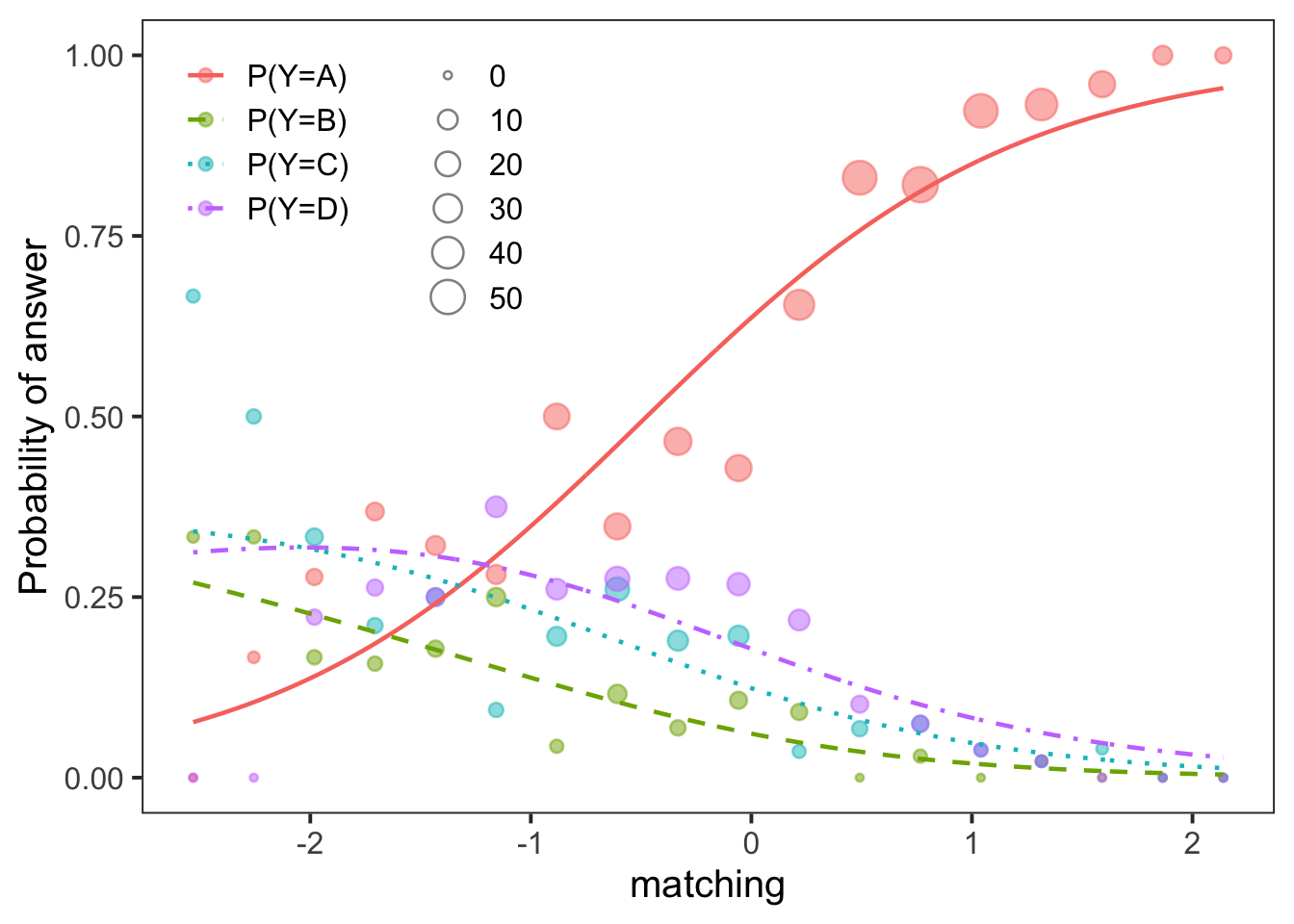
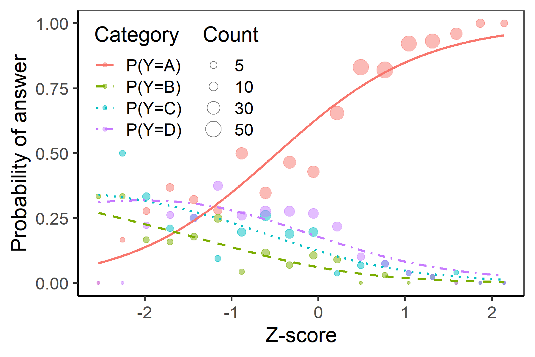
HCItest dataset.
The estimated difficulty (threshold) parameters of \(-1.65\), \(-1.33\), and \(-1.21\), respectively, correspond to the locations for the intersections of the probability curve for the correct answer and the distractors B, C, and D, respectively (Figure 6.9). The slopes describe how flattened the category probability curves are. For each level of ability, the category probabilities again add up to 1.
Instead of fitting a separate model for each single item, a joint model Equation 6.2 may be fitted for all items. This somewhat increases complexity of the estimation process. For example, when using the ML estimation method discussed in Section 4.3 and Section 6.5.2, the joint likelihood function analogous to Equation 6.13 will have the form
\[ L(\boldsymbol{\xi}) = \prod_{p = 1}^n \prod_{i = 1}^m \pi_{pi}^{y_{pi}} \left(1 - \pi_{pi}\right)^{1 - y_{pi}}, \]
where \(\boldsymbol{\xi}\) is now a matrix containing item parameters for all items.
Joint model in R. As an example, we again consider items of the HCI test in a long format – the HCIlong dataset. The joint 1PL model may be fitted with the glm() function to the model variable rating, i.e., item score, on identifiers of items (item) excluding intercept term (using syntax -1). The joint 1PL model moreover includes zscore as a covariate:
fit_1PL_joint <- glm(rating ~ -1 + item + zscore, data = HCIlong,
                     family = binomial)
coef(fit_1PL_joint)
itemItem 1 itemItem 10 itemItem 11 itemItem 12 itemItem 13 itemItem 14
1.0097867 0.7318226 1.5032897 0.3465571 0.5243844 1.3712583
itemItem 15 itemItem 16 itemItem 17 itemItem 18 itemItem 19 itemItem 2
-0.2851713 0.5165578 -1.0489680 1.6320635 1.5454141 1.3319860
itemItem 20 itemItem 3 itemItem 4 itemItem 5 itemItem 6 itemItem 7
1.1436565 2.0333493 -0.4829168 -0.2927134 -0.6936697 0.2174287
itemItem 8 itemItem 9 zscore
1.0449487 -0.3380549 0.9860873 The joint slope parameter is \(0.99\) which is close to 1 (Figure 6.10 (a)).
Similarly, a 2PL model may be fitted including, instead, an interaction between the standardized score and identifiers of the items (term zscore:item):
fit_2PL_joint <- glm(rating ~ -1 + item + zscore:item, data = HCIlong,
                   family = binomial)
coef(fit_2PL_joint)
itemItem 1 itemItem 10 itemItem 11 itemItem 12
1.0117523 0.7138519 1.5345362 0.3508114
itemItem 13 itemItem 14 itemItem 15 itemItem 16
0.5552228 1.4739497 -0.2879333 0.5586961
itemItem 17 itemItem 18 itemItem 19 itemItem 2
-0.8941163 2.0232170 1.7477769 1.2723254
itemItem 20 itemItem 3 itemItem 4 itemItem 5
1.2136989 2.3746433 -0.4340269 -0.2872576
itemItem 6 itemItem 7 itemItem 8 itemItem 9
-0.7498113 0.1972081 1.0866928 -0.3114368
itemItem 1:zscore itemItem 10:zscore itemItem 11:zscore itemItem 12:zscore
0.9925135 0.9006916 1.0535165 1.0328519
itemItem 13:zscore itemItem 14:zscore itemItem 15:zscore itemItem 16:zscore
1.1824314 1.2166280 1.0092705 1.2542630
itemItem 17:zscore itemItem 18:zscore itemItem 19:zscore itemItem 2:zscore
0.3843564 1.6574656 1.3747664 0.8293761
itemItem 20:zscore itemItem 3:zscore itemItem 4:zscore itemItem 5:zscore
1.1766370 1.4841545 0.6751106 0.9399246
itemItem 6:zscore itemItem 7:zscore itemItem 8:zscore itemItem 9:zscore
1.1988226 0.4930918 1.1129665 0.7689954 The estimated slopes differ for each item (Figure 6.10 (b)). For item 13, the intercept parameter estimate of 0.56 and the slope parameter of 1.18 are almost identical to estimates obtained with the logistic regression model fit2PL for a single item in Section 6.4.1.
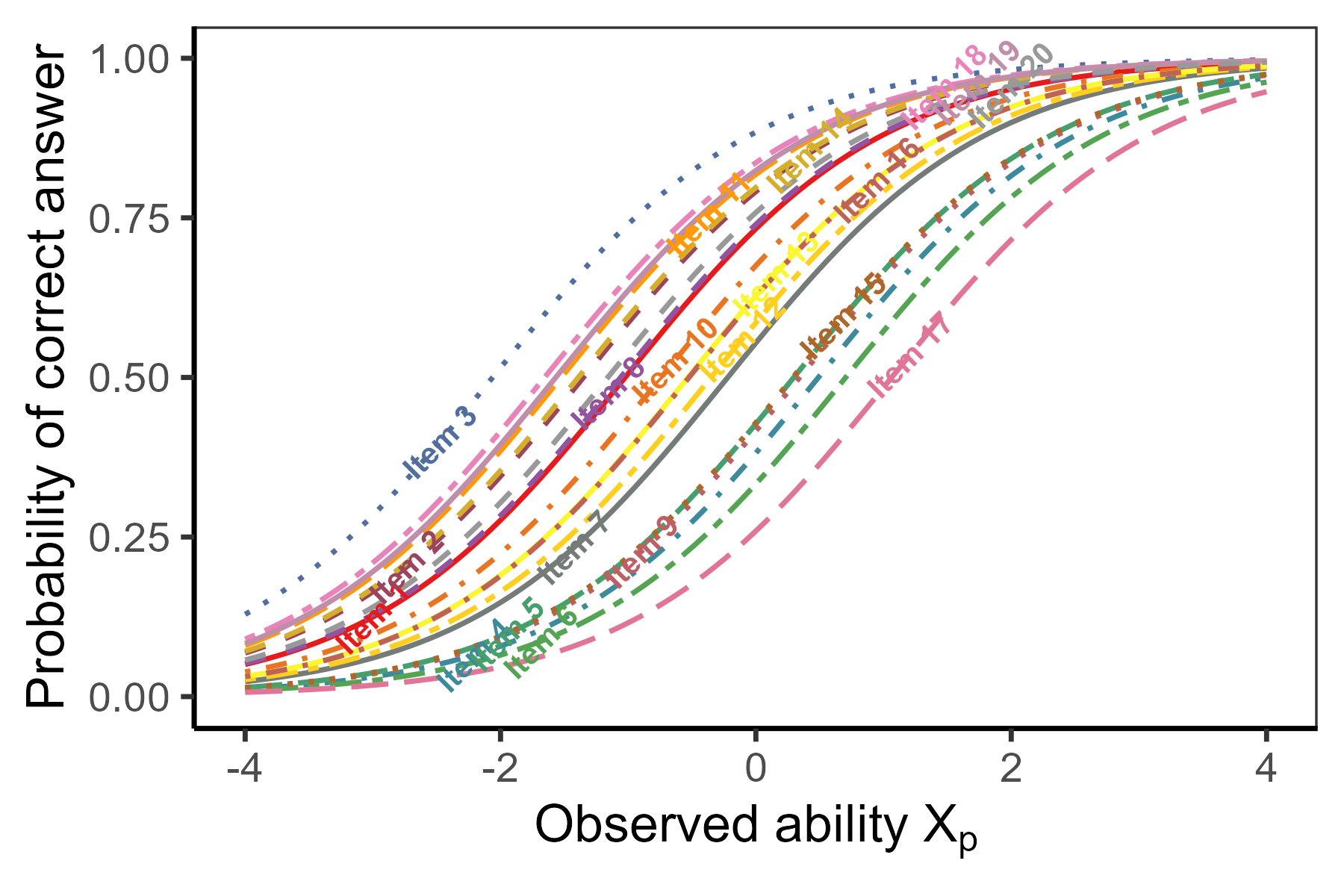
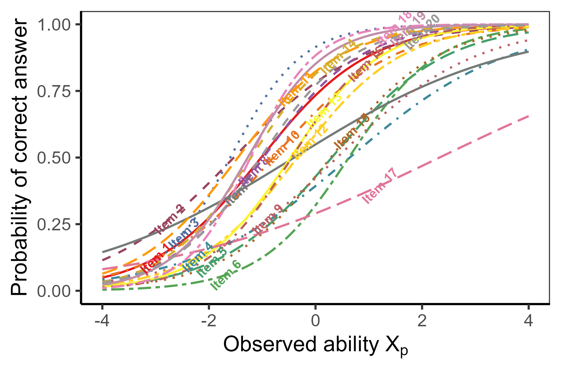
HCIlong dataset.
The models are compared using the LRT Equation 2.29, the AIC Equation 6.15, and the BIC Equation 6.16.
anova(fit_1PL_joint, fit_2PL_joint, test = "LRT")Analysis of Deviance Table
Model 1: rating ~ -1 + item + zscore
Model 2: rating ~ -1 + item + zscore:item
Resid. Df Resid. Dev Df Deviance Pr(>Chi)
1 12999 13790
2 12980 13632 19 157.04 < 2.2e-16 ***
---
Signif. codes: 0 '***' 0.001 '**' 0.01 '*' 0.05 '.' 0.1 ' ' 1AIC(fit_1PL_joint, fit_2PL_joint) df AIC
fit_1PL_joint 21 13831.46
fit_2PL_joint 40 13712.43BIC(fit_1PL_joint, fit_2PL_joint) df BIC
fit_1PL_joint 21 13988.42
fit_2PL_joint 40 14011.40In this case, the p-value far below \(0.05\) with the LRT as well as the smaller AIC suggest the most complex 2PL model fits better on items of the HCIlong dataset. The BIC suggests that the 1PL model, with a common slope, is the better fitting model.
The joint regression model allows for displaying the person scores (observed abilities) and item difficulties on the same scale in a so-called person-item map, also called a Wright map. The map displays the histogram of observed abilities on the left and the items on the right. The location of each item corresponds to the ability level at which the probability of answering the item correctly (or endorsing the item) is exactly 0.5.
Person-item map in the ShinyItemAnalysis package. To plot the person-item map, we use the ggWrightMap() function of the ShinyItemAnalysis package, and we specify the variable for the person abilities (Z-scores for the HCI dataset) through the argument theta and for the item difficulties calculated based on the 1PL model fit_1PL_joint through the argument b. We use the argument ylab.theta to replace the default setting of the left y-axis label.
ggWrightMap(theta = HCI$zscore, b = -coef(fit_1PL_joint)[1:20],
            ylab.theta = "Respondent Z-score")
In this case, a score of about 1 SD below the mean (Z-score of \(-1\)) is needed to correctly answer item 1 with a probability of 0.5 (Figure 6.11 (a)).
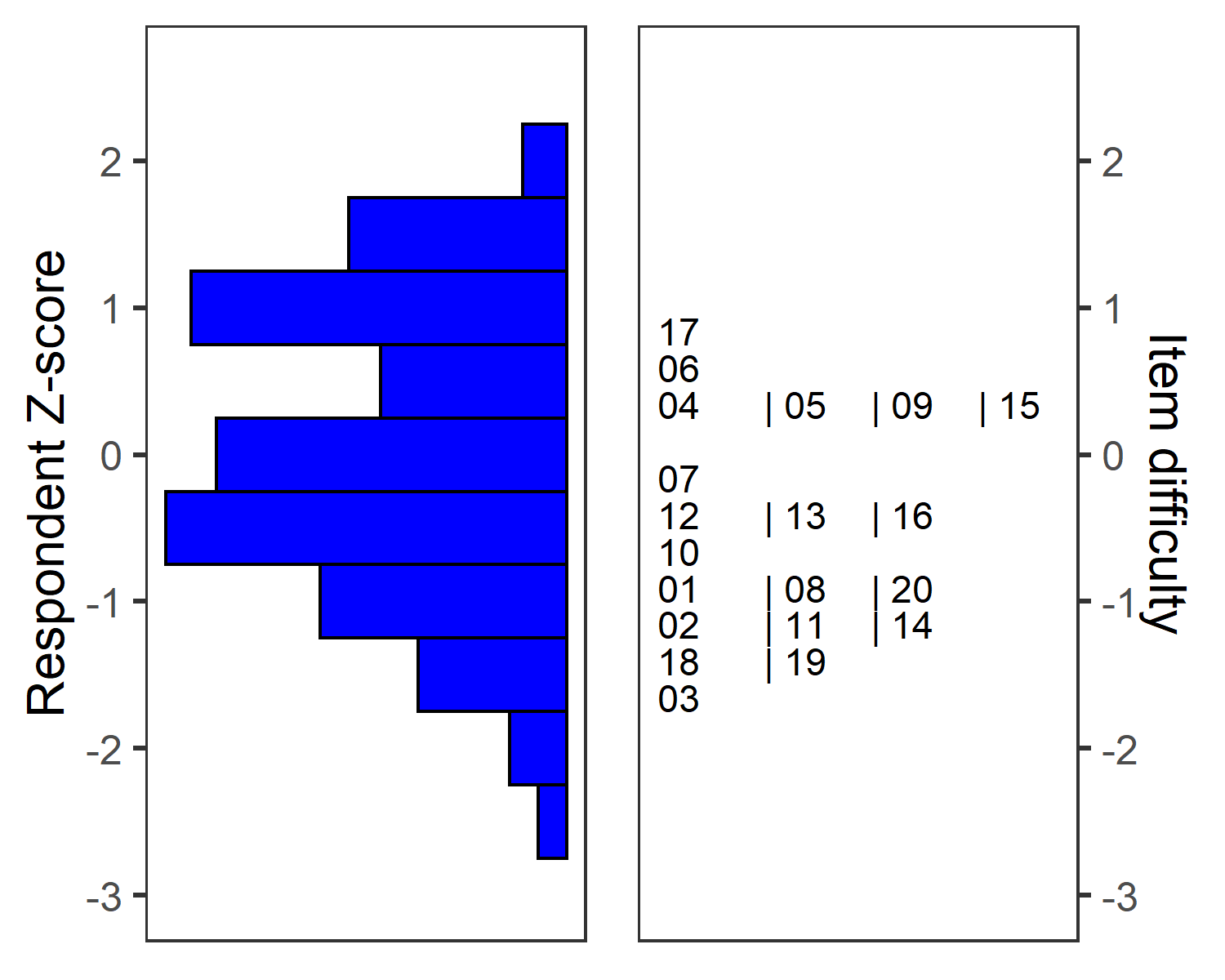
HCI dataset
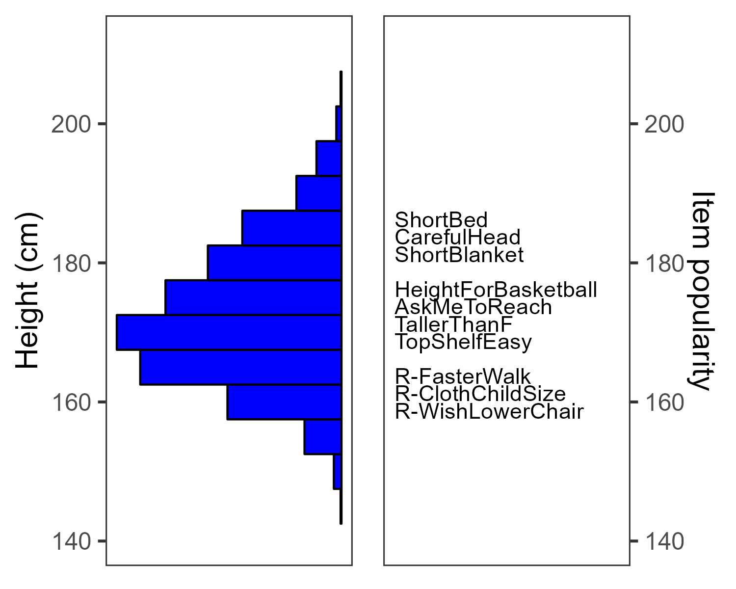
HeightInventory dataset
HCI dataset and the HeightInventory dataset. Left: Distribution of Z-scores or heights. Right: Items, located at the level (Z-score or height) for which the estimated probability of agreeing to that item is 0.5.
To further explore the possibilities of the ggWrightMap() function, we will create one more person-item map now for the HeightInventory dataset. We use the real height as the independent variable and we add labels of the items (see Supplementary code). Item “Ordinary beds are too short for me” labeled as ShortBed is the least popular item; height of about 185 cm is needed to agree with that item with a probability 0.5 (Figure 6.11 (b)). We will return to this example in the next chapter.
The Regression section of the ShinyItemAnalysis application allows for modeling of item properties with logistic, non-linear, ordinal, or multinomial regression models. Individual tabs offer plots of fitted probability curves with empirical values presented by points, equation of the model, and the table of estimated parameters, as well as their brief interpretation (Figure 6.12).
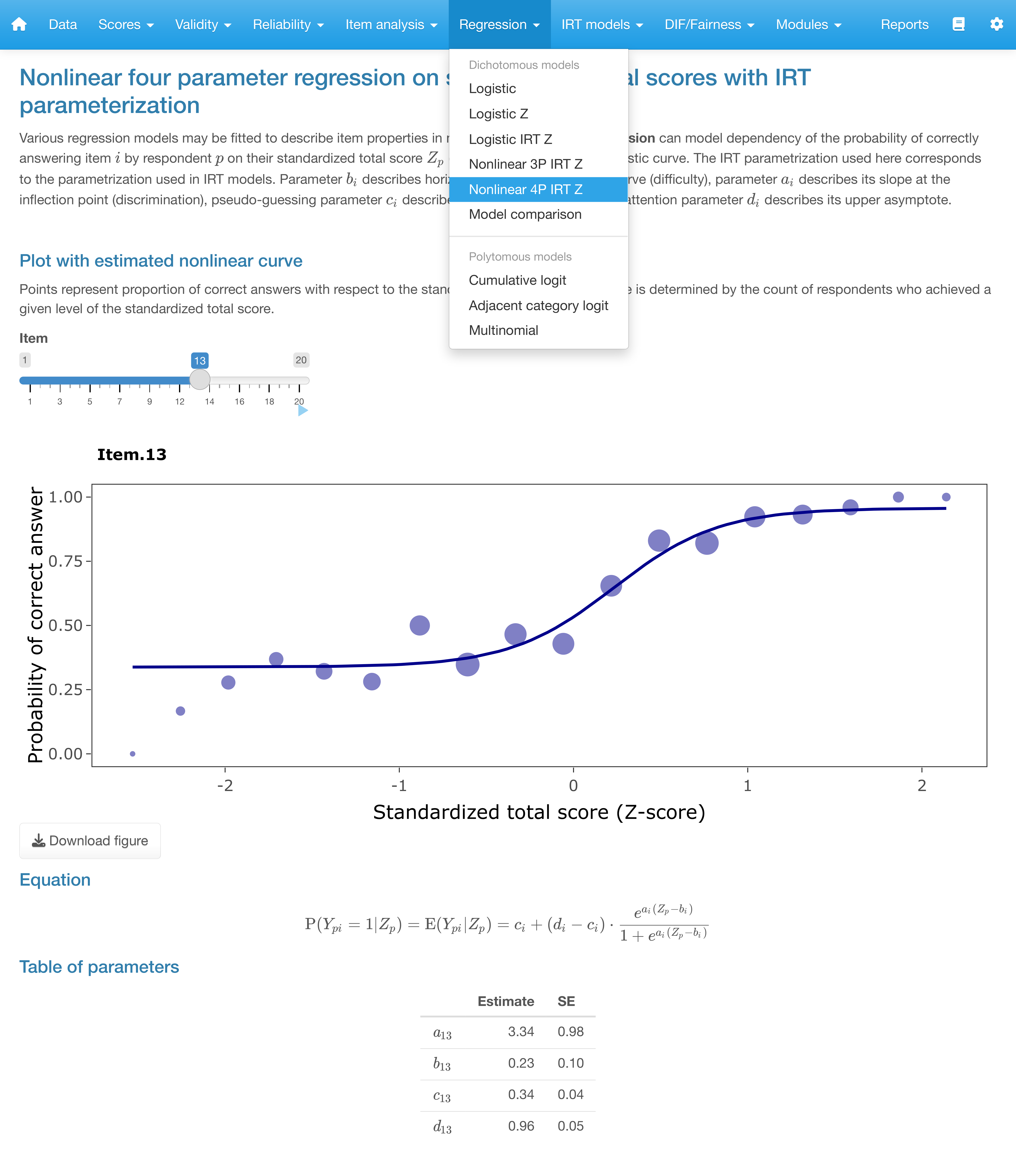
ShinyItemAnalysis.
Binary models start with the classical parametrization and total test scores as a regressor. Then the Regression tab offers models on Z-scores, and models using the IRT parametrization. The logistic regression models are then generalized by introducing the probability of guessing with the 3PL model Equation 6.11. Finally, application offers the 4PL model Equation 6.12 accounting for a respondent’s inattention when answering binary items. The model fit can be statistically compared by AIC or BIC in the Model comparison tab.
For ordinal data, cumulative logit Equation 6.18 and adjacent-categories logit Equation 6.22 models are offered in relevant tabs. The tab Cumulative logit provides two plots – a plot of cumulative and a plot of category probabilities.
Finally, nominal items can be analyzed using the multinomial regression model Equation 6.25. For all three models, observed score can be selected directly within the tab. Moreover, the tabs offer the possibility to select either the classical intercept-slope parametrization or the IRT parametrization. Corresponding plot, estimates of parameters, and interpretation are displayed interactively for the selected item based upon the user’s choice.
In this chapter, we have presented regression models for a description of item functioning in multi-item measurements. The presented models assumed that the trait of interest is directly available and does not contain any measurement error, an assumption which will be relaxed in subsequent chapters. Models for continuous, binary, ordinal, and nominal items were presented. We have then discussed estimation of model parameters, model selection, and model fit. While most of the chapter considered analysis of single items, we have also presented joint models for all items. The final section offered analysis in interactive application.