7 Item response theory models
7.1 Introduction
In Section 9.4, we used regression models to describe the properties of items in multi-item instruments with respect to a directly available trait. For example, in the HeightInventory dataset, respondents were asked questions related to their height, while their actual height (in centimeters) was also provided. Difficulty and more detailed functioning of each item in the HeightInventory dataset was analyzed using a regression model predicting the respondent’s score on each item by their height.
We utilized the fact that height was directly available, and we assumed it did not contain any measurement errors. However, in situations typically encountered in psychometrics, the trait is typically unobserved and the multi-item instrument itself needs to be used to estimate it.
In this chapter, we present latent variable models termed item response theory (IRT) models which allow us to jointly model and estimate the item parameters and the respondent latent traits (person parameters). The additional complexities of IRT models have several advantages. First, as with the regression models presented in Section 9.4, it is possible to enumerate the precision of the item parameters and to thusly describe item functioning, in more detail for all levels of the latent traits by using a smooth curve. The latent trait will, however, no longer be able to be directly observed and we will be able to estimate item parameters based solely upon item responses. Moreover, the IRT models focus upon the estimation of a latent trait (ability) itself. The precision of the ability estimate is therefore also of interest, and test reliability is studied in greater detail as a function of ability.
As with the regression models in Section 9.4, the estimated latent trait will share the same scale as the item parameters. While the scale was directly available previously, it is now driven by item responses, and additional restrictions need to be established to assure parameters are identified. As observed in the person-item map, introduced in Section 6.8.1, when the regression model is used, the item parameters can be interpreted with respect to real height in centimeters. This is in contrast to the IRT model where the origin and scale of the latent trait are defined rather arbitrarily, and its mean is often fixed at 0 and its variance at 1 (Figure 7.1).
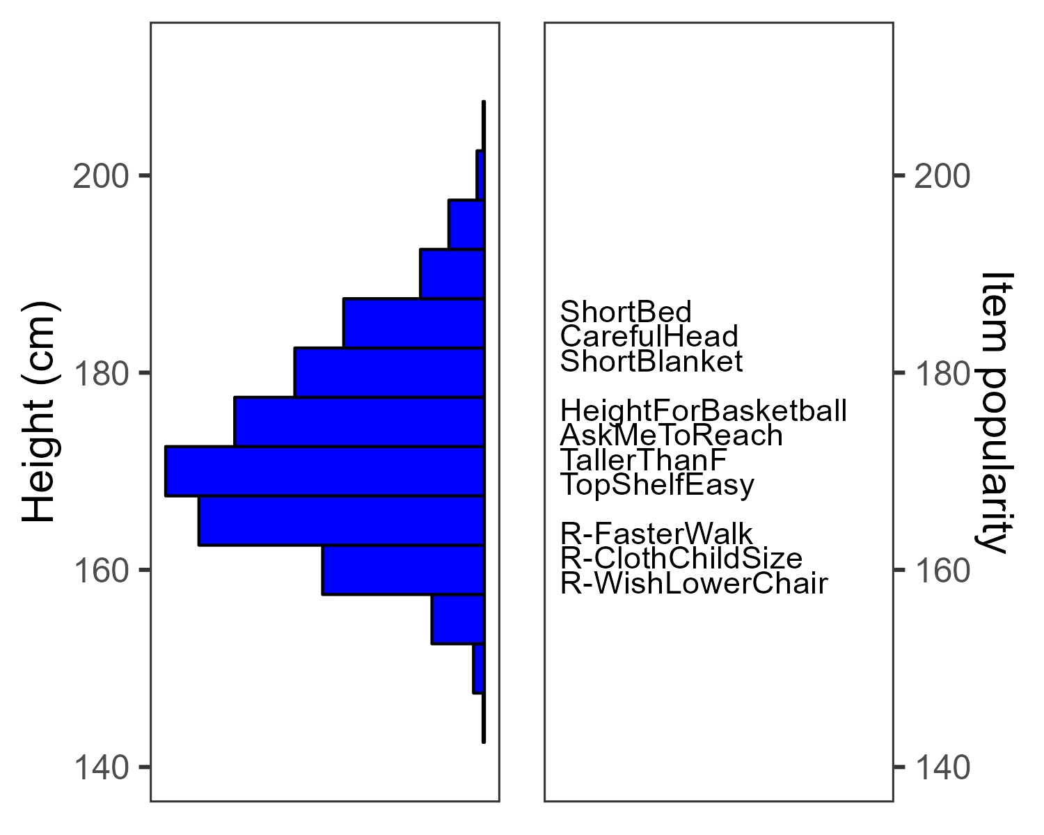
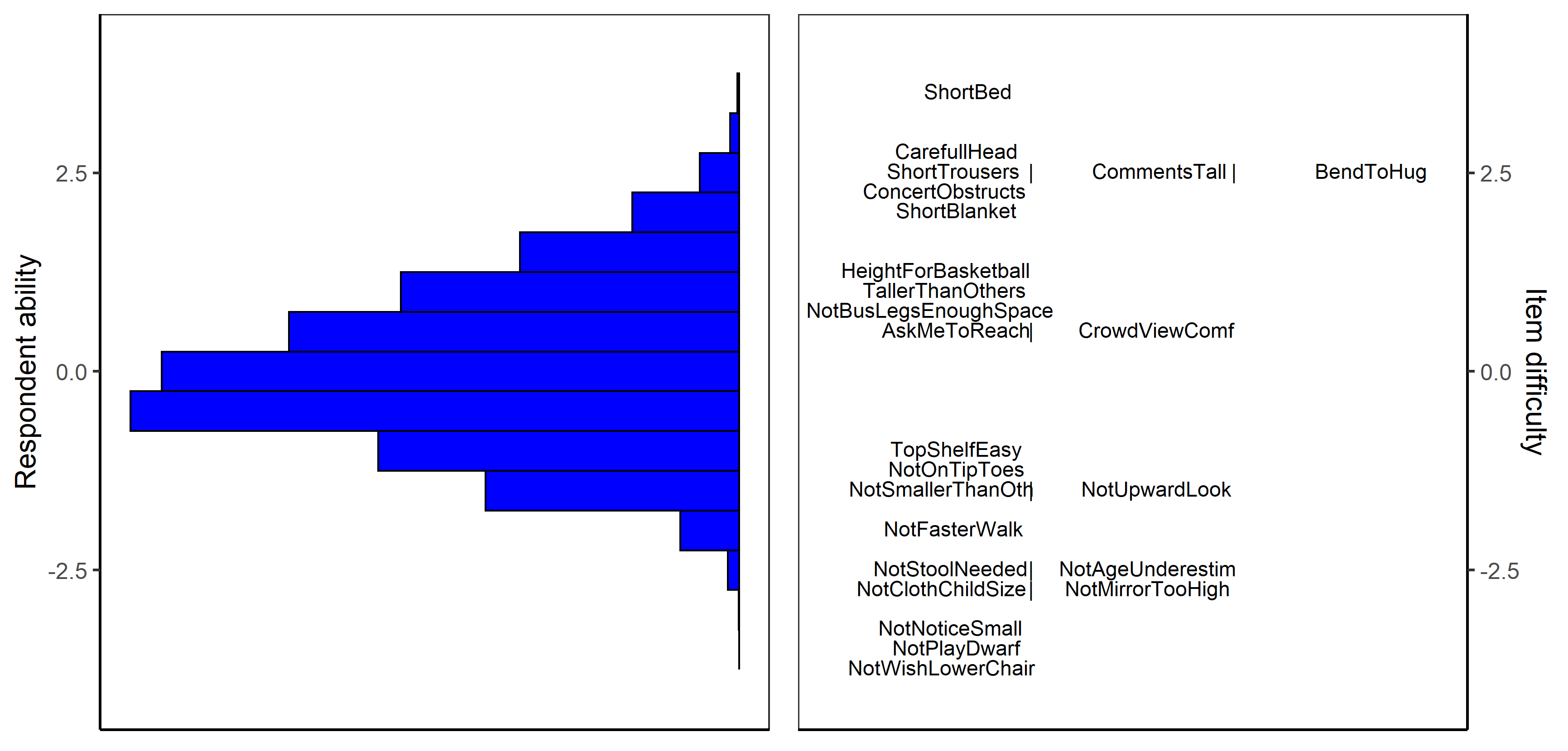
HeightInventory dataset. Left panels: Distribution of (latent) heights. Right panels: Items, located at the level of (latent) height for which the estimated probability of agreeing to that item is 0.5. For better readability, only the selection of item labels is displayed.
For example, when the height of respondents is available in the dataset, the regression model predicts that a height of about 180 cm is needed to agree with the item “Blankets and bedspreads rarely cover me completely” with a probability of 0.5 (Figure 7.1 (a)). The IRT model predicts that a height of about 0.8 SD above the mean is needed to agree with this ShortBlanket item with a probability of 0.5 (Figure 7.1 (b), see Exercise 7.4 for sample R code). If the population mean and standard deviation of the real height in centimeters are available, we can eventually end up with analogous information as if the height was actually measured in centimeters, but in psychological measurement this is typically not the case.
This chapter proceeds as follows: We will start with general concepts, assumptions, and different IRT models for binary data in Section 7.2. We will then discuss the estimation of item parameters and an estimation of the respondent level of a latent trait in Section 7.3. Once these concepts are covered, we will turn our attention to the comparison of different R packages for an estimation of IRT models in Section 7.4, while implementation of the interactive ShinyItemAnalysis application is described in Section 7.6.
Throughout this chapter, we will conceptualize the IRT models as Generalized Linear Mixed Effect Models (GLMMs) or nonlinear mixed effect models (Rijmen et al., 2003). We chose this framework because it follows directly from the Generalized Linear Models (GLMs) and nonlinear regression models for item description built in Section 9.4. The main difference is that, while in GLMs the respondent abilities are directly available and treated as fixed effects, in GLMMs, the abilities are treated as unobserved/latent scores \(\theta\) and modelled as random effects following a certain distribution. Later, in Section 7.5, we will discuss how IRT models can be conceptualized within the framework of factor analysis introduced earlier in Chapter 2.
While in this chapter we will explain the general concepts and IRT models for binary data, in Chapter 8 we will discuss extensions of more complex IRT models, including those for polytomous items or multidimensional latent traits. For further details on IRT models, the reader is referred to Debelak et al. (2022) or Linden (2017).
7.2 General concepts and assumptions
7.2.1 IRT model assumptions
The basic IRT models have several assumptions which we will investigate and build upon throughout the next sections of this chapter and in following chapters.
Dimensionality of a latent trait. The first assumption concerns the continuous latent trait \(\theta\) which is driving the respondents’ answers. The assumption of unidimensionality means that the instrument measures a single construct. This is plausible, e.g., when measuring knowledge of algebra or the level of a patient’s fatigue or pain. Multidimensional traits are more common in psychological measurement and personality research, but a mathematics test may also be measuring two-dimensional ability (e.g., computing skills and reading comprehension) if a notable portion of the questions includes word problems. We have already discussed in Chapter 3 how plausibility of the unidimensionality assumption can be checked. In a case where the unidimensional latent trait cannot be expected, multidimensional IRT models are more appropriate (see Chapter 8).
Functional form of the latent variable model. The core of IRT models is the formula which prescribes the probability of a given response \(y_{pi}\) as a function of the respondent’s location on the latent continuum \(\theta_p\) and of a certain set of item parameters \(\boldsymbol{\xi}_i\) (such as item difficulty or discrimination) which are to be estimated. \[ \Pr(Y_{pi} = y_{pi}| \theta_p, \boldsymbol{\xi}_i) = f(Y_{pi}, \theta_p, \boldsymbol{\xi}_i). \] This function is often denoted as an item response function (IRF), and when plotted out, it is termed an item response curve (IRC). In Section 9.5.1 below, we will describe the IRFs of the most common IRT models for binary items. The functional form is similar to the regression models described in Section 9.4, with the main difference being the treatment of the respondent’s ability, which in Section 9.4 was represented by an observed variable \(X_p\) that is modelled using a fixed effect, while in IRT it is an unobserved, latent variable \(\theta_p\) which needs to be estimated.
While IRF describes individual responses, the item characteristic function (ICF) describes the expected score on the item: \[ \text{E}(Y_{pi}| \theta_p, \boldsymbol{\xi}_i) = \int y_{pi} f(y_{pi}| \theta_p, \boldsymbol{\xi}_i) \, \mathrm{d} y_{pi}. \] The graphical representation of the ICF is the item characteristic curve (ICC). The ICF is often assumed to be a monotone function: For example, in educational tests we expect that the mean score will be higher with a higher level of ability. For binary items, the IRF of the correct answer is equal to the ICF, because the mean score is simply equal to the probability of a correct answer: \[ \text{E}(Y_{pi}| \theta_p, \boldsymbol{\xi}_i) = 1 \cdot \Pr(Y_{pi} = 1| \theta_p, \boldsymbol{\xi}_i) + 0 \cdot \Pr(Y_{pi} = 0| \theta_p, \boldsymbol{\xi}_i) = \Pr(Y_{pi} = 1| \theta_p, \boldsymbol{\xi}_i). \] In binary models, the terms IRF and ICF can thus be used interchangeably. In ordinal items, the IRF and ICF are not the same; see Chapter 8.
To define the properties of the test as a whole, the IRFs of individual items are combined into the test score function (TSF) describing expected test score:
\[ \text{E}\left(\sum_{i = 1}^m {Y_{pi}}\Bigg| \theta_p, \boldsymbol{\xi}\right) = \sum_{i = 1}^m \text{E}({Y_{pi}}| \theta_p, \boldsymbol{\xi}_i), \]
which is graphically represented with the test score curve (TSC).
Independence of respondents. In a typical setting it is assumed that the respondents’ answers to an item are independent. In an educational context, violation of this assumption can be expected when the respondents are clustered in classrooms, schools, towns, and/or countries. The correlation structure of the data can then be accounted for by using hierarchical IRT models.
Conditional independence of item scores. The next critical assumption of IRT models is that given the respondents’ latent traits, their item responses are conditionally independent. In other words, we typically assume that the respondent’s response to one item is not dependent on responses to other items in ways other than through their ability. This assumption is termed conditional independence or local independence.
For example, assume respondent \(p\) with ability \(\theta_p\) answered correctly to binary items 1 and 2 with probabilities \(\Pr(Y_{p1} = 1 | \theta_p, \boldsymbol{\xi}_{1}) = \pi_1\) and \(\Pr(Y_{p2} = 1 | \theta_p, \boldsymbol{\xi}_{2}) =\pi_2\). The probabilities of incorrect answers are \(1 - \pi_1\) and \(1 - \pi_2\), respectively. The conditional independence assumption then directly implies the probabilities of all possible response patterns. For example, the probability of response pattern \((1, 0)\), i.e., answering the first item correctly and the second one incorrectly, is the product of the two probabilities: \[ \Pr(Y_{p1} = 1, Y_{p2} = 0| \theta_p, \boldsymbol{\xi}_{1}, \boldsymbol{\xi}_{2}) = \pi_1 (1 - \pi_2). \] Conditional independence is a key assumption for a straightforward calculation of likelihood as a product of probabilities which is used in parameter estimation (see Section 7.3).
The assumption of conditional independence is typically violated in competence tests where a bundle of items is connected to one reading passage or graph. In such cases, more complex IRT models are needed.
Invariance of item parameters. Under the assumption of item parameter invariance, the estimated item parameters are about the same in subsamples of respondents. This assumption is violated in a case of DIF (see Chapter 9), i.e., in a situation when an item functions differently for different groups of respondents. More complex, group-specific models are needed if assumption of item parameter invariance does not hold.
7.2.2 IRT models for binary data
IRT models for binary data can be conceptualized as counterparts of GLMs, such as logistic or probit regression models, described in Section 6.4.
7.2.2.1 Rasch or 1PL IRT model
The Rasch model (Rasch, 1960) is very simple in its form. It assumes discrimination of all items is equal to one. The assumption of common discrimination is plausible, for example, in a test of mathematics involving a series of items testing the same mathematical operation but using different numbers – free throws in basketball using different distances from the basket, a high jump with different heights of the bar, or repeated chess matches against computer programs of different strengths (Davier, 2016).
The Rasch model can be defined as
\[ \pi_{pi} = \Pr(Y_{pi} = 1|\theta_p) = \frac{\exp(\theta_p - b_i)}{1 + \exp(\theta_p - b_i)}. \tag{7.1}\]
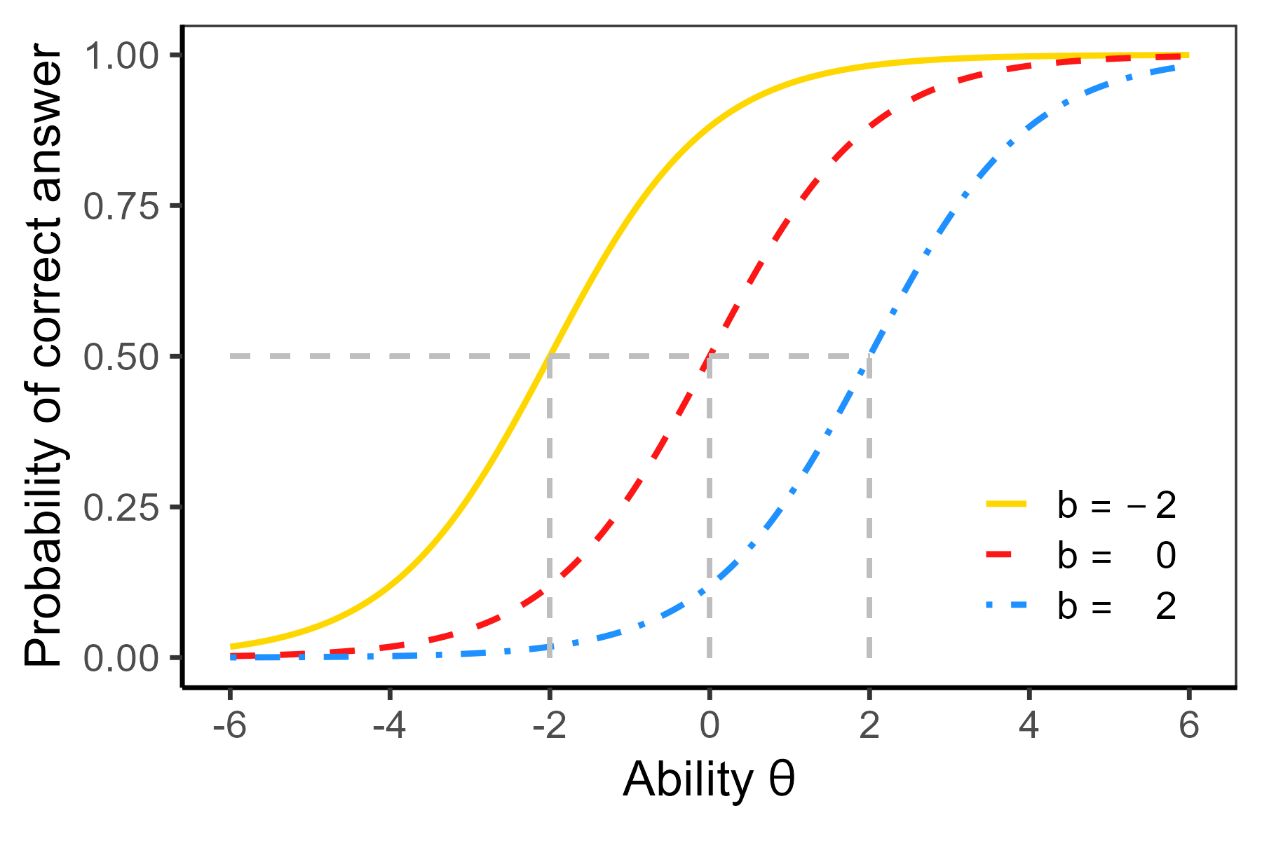
In this equation, \(\theta_p\) is a trait of person \(p\) which is often assumed to follow normal distribution \(\mathcal{N}(0, \sigma^2)\) with variance \(\sigma^2\). Parameter \(b_i\) is the difficulty of item \(i\), which describes the location of an inflection point of the ICC. It is also the ability level for which the probability of endorsing the item is equal to \(0.5\) (Figure 7.2 (a)).
As with the logistic regression model Equation 6.5, the logit of the probability for a correct answer is a linear function of the ability
\[ \textrm{logit}(\pi_{pi}) = \log\left(\frac{\pi_{pi}}{1 - \pi_{pi}}\right) = \theta_p - b_i, \tag{7.2}\]
which makes this model belong to the class of GLMM.
A 1PL IRT model is equivalent to the Rasch model, but is usually parametrized so that item discrimination \(a\) is relaxed in any real number, while it is still assumed to be constant across items, \(\textrm{logit}(\pi_{pi}) = a(\theta_p - b_i)\). This comes with a restriction to the ability variance of one, \(\sigma^2 = 1\). Under the 1PL model, the ability is then typically assumed to follow a standard normal distribution \(\mathcal{N}(0, 1)\).
7.2.2.2 2PL IRT model
The 2PL IRT model (Birnbaum, 1968) allows for different discriminations of individual items. As such, the model is a counterpart of the logistic regression model Equation 6.8 presented in Section 9.4. It is usually parametrized as
\[ \pi_{pi} = \Pr(Y_{pi} = 1|\theta_p) = \frac{\exp(a_i(\theta_p - b_i))}{1 + \exp(a_i(\theta_p - b_i))}, \tag{7.3}\]
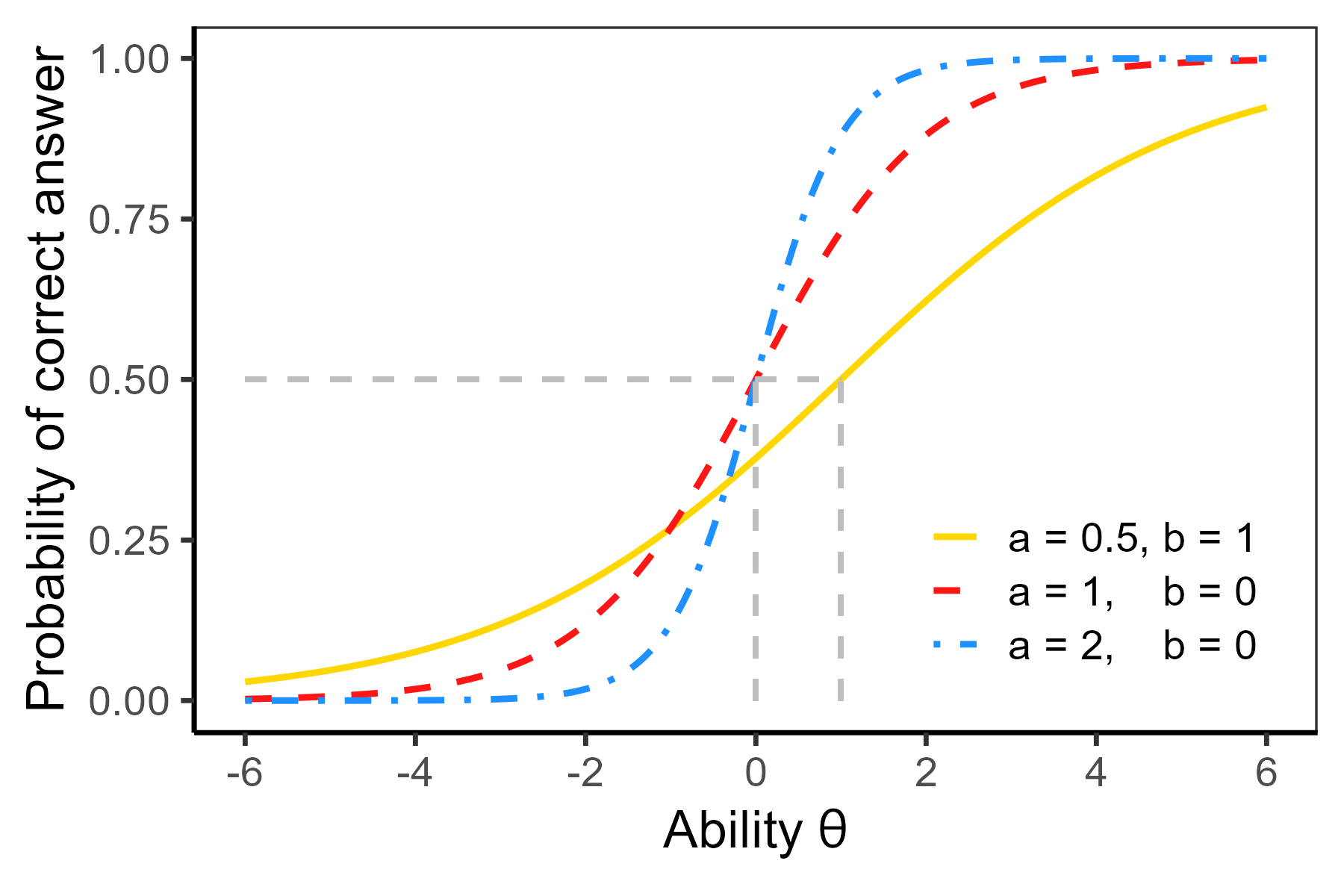
where \(\theta_p\) is a trait of person \(p\) typically assumed to follow a standard normal distribution. Parameter \(b_i\) is item \(i\) difficulty parameter (location of the inflection point), and \(a_i\) is item discrimination parameter, i.e., the slope at the inflection point (Figure 7.2 (b)). See Section 6.4.3 for more detailed derivation of parameter interpretations.
As was the case for the Rasch model Equation 7.2, the 2PL IRT model belongs to the class of GLMMs, given that the logit of the probability of a correct answer is a linear function of the ability, \(\textrm{logit}(\pi_{pi}) = a_i(\theta_p - b_i).\)
7.2.2.3 Normal-ogive model
As was discussed in Section 6.4.2, a probit link may be an alternative to a logit link function in regression models for binary data. The probit IRT model is often called a normal-ogive model (Lord & Novick, 1968), and as a two-parameter model it is defined as
\[ \Pr(Y_{pi} = 1|\theta_p) = \Phi(a_i(\theta_p - b_i)), \tag{7.4}\]
where \(\Phi(x)\) is the CDF for the standard normal distribution Equation C.4.
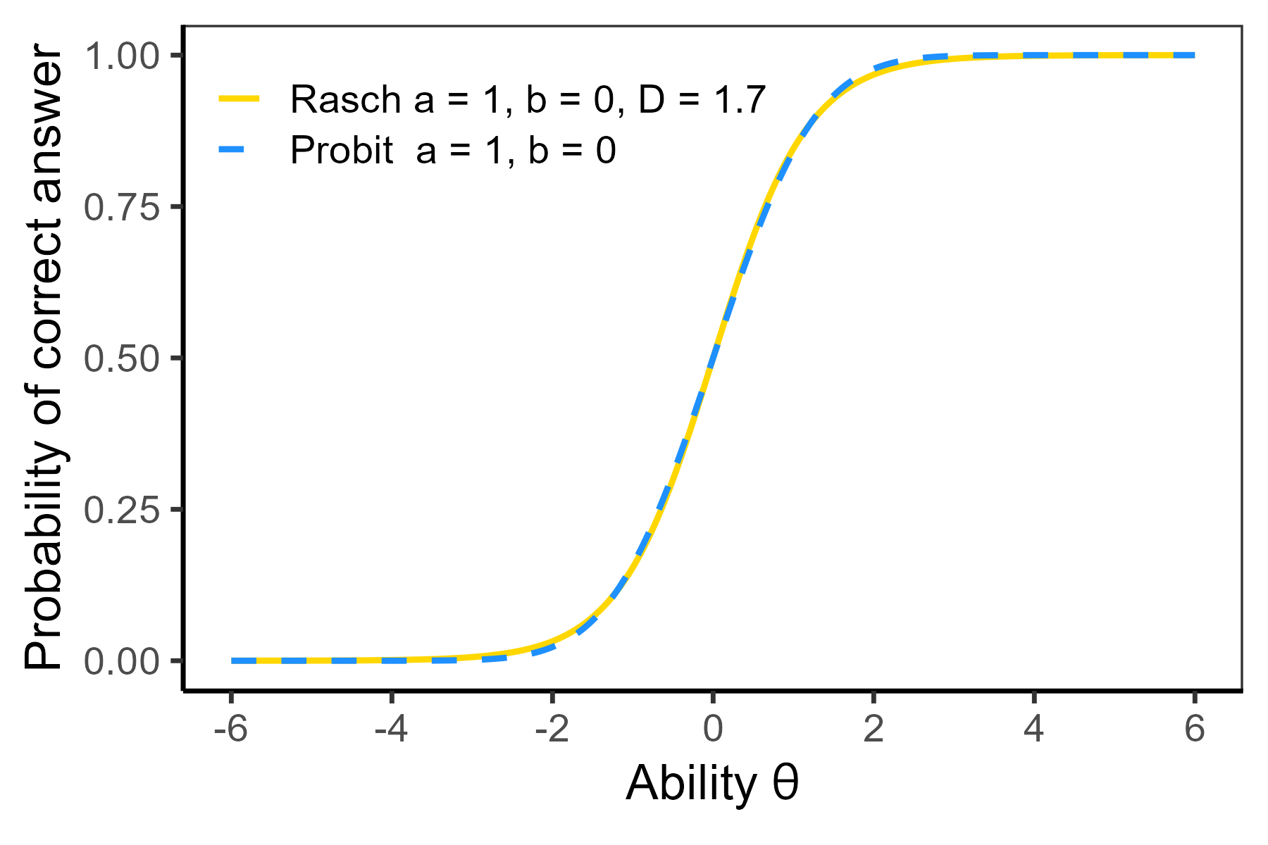
Logistic IRT models are sometimes defined using a scaling parameter \(D = 1.702\), which for the 2PL IRT model Equation 7.3 takes the following form: \[ \Pr(Y_{pi} = 1|\theta_p) = \frac{\exp(D a_i (\theta_p - b_i))}{1 + \exp(D a_i (\theta_p - b_i))}. \] The scaling parameter \(D\) is selected in order to closely match a logistic IRT model with an analogous probit model with the same difficulty and discrimination parameters see also 7.3.
7.2.2.4 3PL IRT model
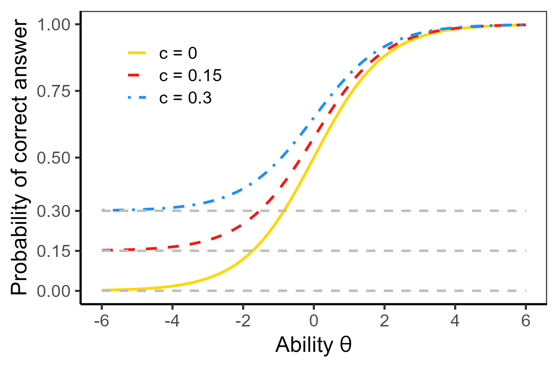
The 3PL IRT model (Birnbaum, 1968) allows for a non-zero lower/left asymptote \(c_i\), which in the context of educational tests may represent item guessing, i.e., the probability with which even a respondent with no ability can answer an item correctly:
\[ \pi_{pi} = \Pr(Y_{pi} = 1|\theta_p) = c_i + (1 - c_i) \frac{\exp(a_i(\theta_p - b_i))}{1 + \exp(a_i(\theta_p - b_i))}. \tag{7.5}\]
This model is a counterpart to the 3PL model Equation 6.11. Unlike the Rasch and the 2PL IRT models, this model does not belong to the class of GLMMs, since there is no link function for the probability of a correct answer, which would be a linear function of the ability. The practical consequence is that the parameter estimation may become more challenging.
Typical values of a guessing parameter are between \(0\) and \(0.35\) (Figure 7.4 (a)), but oftentimes the estimated parameters are even higher. In multiple-choice items, one would expect guessing about \(1/K_i\) with \(K_i\) being the number of response options in item \(i\). However, the distractors (incorrect options) usually have an intrinsic attractiveness; therefore, when freely estimated, the estimates may be further from \(1/K_i\). For this reason, \(c_i\) is often called the pseudo-guessing parameter. With low sample sizes it may be difficult to fit the 3PL model, and it may be helpful to estimate a common pseudo-guessing parameter \(c\), thus restricting model Equation 7.5. Another option is to even fix the pseudo-guessing parameters at \(1/K_i\).
7.2.2.5 4PL IRT model
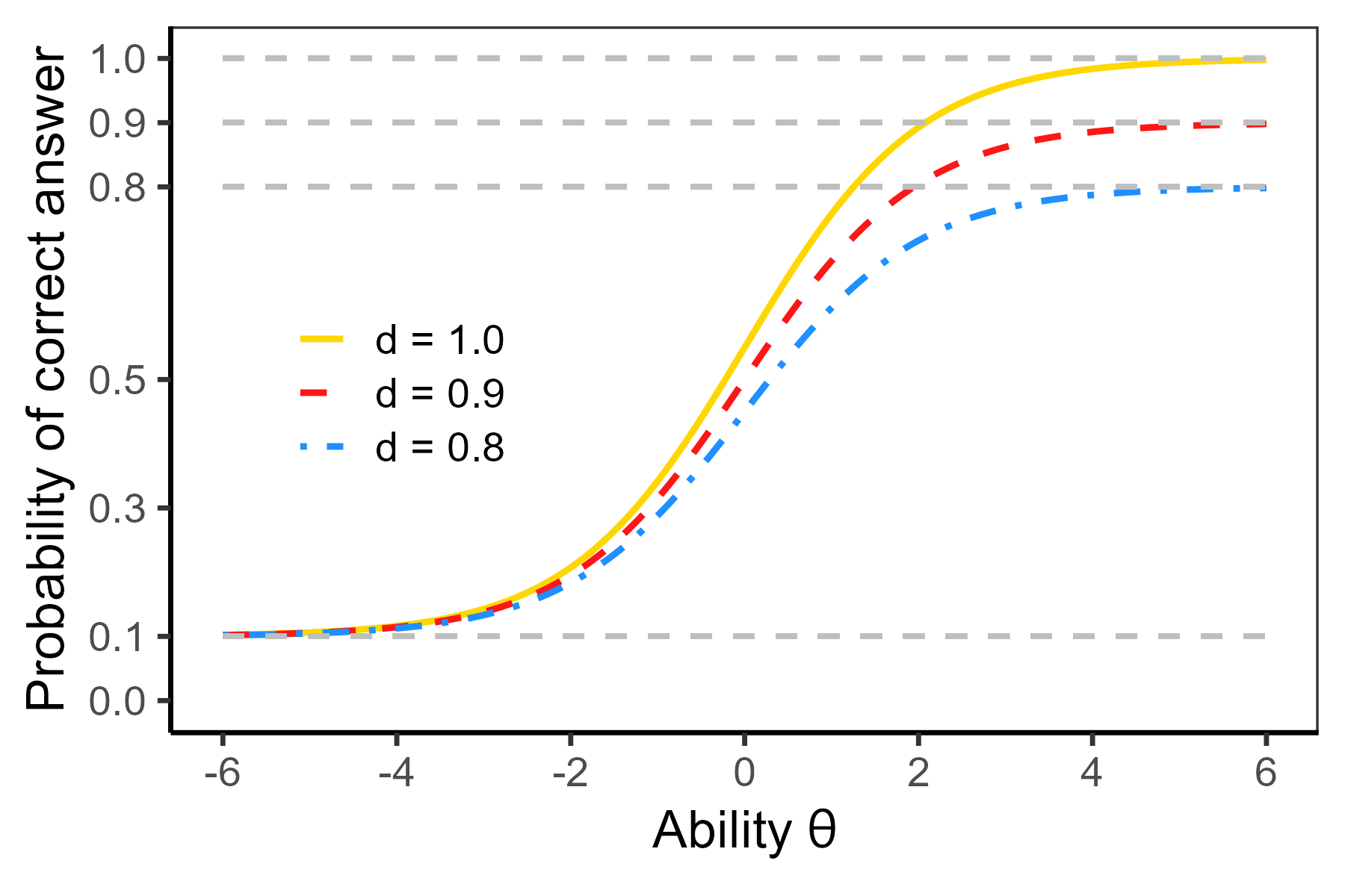
The 4PL IRT model (Barton & Lord, 1981) allows for an upper/right asymptote \(d_i\) lower than 1 (Figure 7.4 (b)). In the context of educational testing, this may represent inattention or slipping: Regardless of how high the respondent’s ability, their probability of a correct answer is still below 1. The 4PL model is defined as
\[ \pi_{pi} = \Pr(Y_{pi} = 1|\theta_p) = c_i + (d_i - c_i) \frac{\exp(a_i(\theta_p - b_i))}{1 + \exp(a_i(\theta_p - b_i))}. \tag{7.6}\]
This model is a latent variable counterpart to the 4PL model Equation 6.12. The Rasch model Equation 7.1 is a special example of the 4PL IRT model with a discrimination parameter fixed at \(a_i = 1\), a pseudo-guessing parameter fixed at \(c_i = 0\), and an inattention parameter (also called slipping parameter) of \(d_i = 1\). Other restricted models (e.g., 2PL and 3PL models) may be obtained by fixing appropriate parameters in the 4PL model Equation 7.6.
In all IRT models presented so far, the intercept-slope parametrization of the IRT models is usually used for parameter estimation:
\[ \pi_{pi} = \Pr(Y_{pi} = 1|\theta_p) = c_i + (d_i - c_i) \frac{\exp(\beta_{0i} + \beta_{1i} \theta_p)}{1 + \exp(\beta_{0i} + \beta_{1i} \theta_p)}, \tag{7.7}\]
where the relationship between the set of parameters is as in Equation 6.9: The slope parameter is equal to the discrimination, \(\beta_{1i} = a_i\) and the intercept is related to item difficulty, \(\beta_{0i} = - a_i b_i\). The standard errors of estimates in the IRT parametrization Equation 7.6 are calculated from standard errors of intercept-slope parametrization Equation 7.7 using the delta method Equation 6.10. The intercept-slope parametrization is also useful for generalizations to multidimensional latent traits (see Chapter 8). Latent ability \(\theta_p\) is usually assumed to follow standard normal distribution \(\mathcal{N}(0, 1)\).
7.3 Estimation methods for IRT models
It is obvious from the previous sections that the key element when fitting the IRT models is the estimation of item and person parameters. Software packages differ in the algorithms that they employ but also in a number of other details. There are several parameter estimation techniques available (Baker & Kim, 2004). Traditional item analysis may provide rough estimates. Most often, estimation is done using ML methods already introduced in Section 6.5. However, in IRT models, both the item and the person parameters need to be estimated, which is solved via JML, MML, or CML. The use of Bayesian methods implementing MCMC have become popular, especially for multidimensional IRT models. We now take a closer look at each of these approaches.
7.3.1 Heuristic methods and starting values
An approximate estimation of item parameters may be obtained from traditional item analysis methods. These heuristic methods are still of great importance, and they provide starting values for numerical algorithms. The choice of starting values is a very important aspect and may have profound impact on the speed of convergence of iterative estimation algorithms, especially in models with a higher number of parameters.
Lord & Novick (1968, 16) showed that under the assumption of a standard normal distribution of the latent trait, and with the normal-ogive 2PL model Equation 7.4, the biserial correlation of item score \(Y_i\) and ability \(\theta\) in the population is related to discrimination parameter \(a_i\): \[ \rho_i = \text{Corr}(Y_i, \theta) = \frac{a_i}{\sqrt{1 + a^2_i}} \textrm{, and thus } a_i = \frac{\rho_i}{\sqrt{1 - \rho_i^2}}; \] thus the sample RIT, introduced in Chapter 5, might be used to estimate the item discrimination \(a_i\), whereas, the proportion of correct answers can be used to estimate the difficulty parameter \(b_i\), because under the normal-ogive 2PL model Equation 7.4 \[ b_i = \frac{\Phi^{-1}(\pi_i)}{\rho_i}, \] with \(\Phi^{-1}\) being the inverse of the CDF of the standard normal distribution Equation C.4.
Other starting values are possible as well. For example, Hladká & Martinková (2020) proposed using adjusted ULI, i.e., difference in proportion of correct answers between upper and lower ability groups, to provide initial estimates of item discrimination parameter in models accounting for asymptotes within the difNLR package.
7.3.2 Joint maximum likelihood
In the case of a unidimensional binary IRT model with a set of item parameters \(\boldsymbol{\xi}\) and a set of latent abilities \(\boldsymbol{\theta}\), the joint likelihood has the following form
\[ L(\boldsymbol{\xi}, \boldsymbol{\theta}) = \Pr(\boldsymbol{Y} = \boldsymbol{y}|\boldsymbol{\theta}, \boldsymbol{\xi}) = \prod_{p = 1}^n \prod_{i = 1}^m \pi_{pi}^{y_{pi}} (1 - \pi_{pi})^{1 - y_{pi}}, \tag{7.8}\]
where \(\pi_{pi}\) is in the form of model Equation 7.7 or of one of its restricted versions.
The idea behind the JML method is to jointly estimate the ability and item parameters in a single iterative algorithm. It typically starts with an initial estimate of item parameters using a heuristic method, and it maximizes the likelihood with respect to ability parameters while considering the item parameters as fixed. Subsequently, the ability parameters will be considered fixed, and the item parameters are updated to values maximizing the likelihood, as was already described in Section 6.5. This algorithm is iterated until a predefined convergence criterion is met.
As was outlined in Section 6.5, the ML algorithm looks for parameters which maximize the likelihood function, or its logarithm, which is mathematically more tractable
\[ \log(L(\boldsymbol{\xi}, \boldsymbol{\theta})) = \sum_{p = 1}^n \sum_{i = 1}^m \left[y_{pi} \log(\pi_{pi}) + (1 - y_{pi}) \log(1 - \pi_{pi})\right]. \tag{7.9}\]
The model is not identified; i.e., there exists no unique solution to the maximization. The indeterminacy of parameter estimates in the origin and unit is typically solved by further constraints: For example, in each step of the algorithm, centering of the person parameters is applied (i.e., setting the mean of the person parameters to zero and the standard deviation to one in 1PL–4PL models), and subsequently item centering is also applied (i.e., setting the mean of item parameters to zero and the standard deviation to one).
Example: Estimating ability parameters with the JML algorithm. To demonstrate in more detail how the ability parameters are estimated with the JML, assume an instrument composed of 5 items following the Rasch model is being answered by 20 respondents. The initial estimate of item difficulty is obtained from the ratios of correct answers \(b_1 = -1.90, b_2 = -0.60, b_3 = -0.25, b_4 = 0.30,\) and \(b_5 = 0.45\). Assume a respondent has a response pattern 11000, i.e., answering the first two items correctly and the last three items incorrectly. How likely is an average respondent (\(\theta_p = 0\)) to produce these responses? How likely is a weaker respondent (\(\theta_p = -1\)) to produce these responses? And most importantly, a respondent with what ability is most likely to produce these responses?
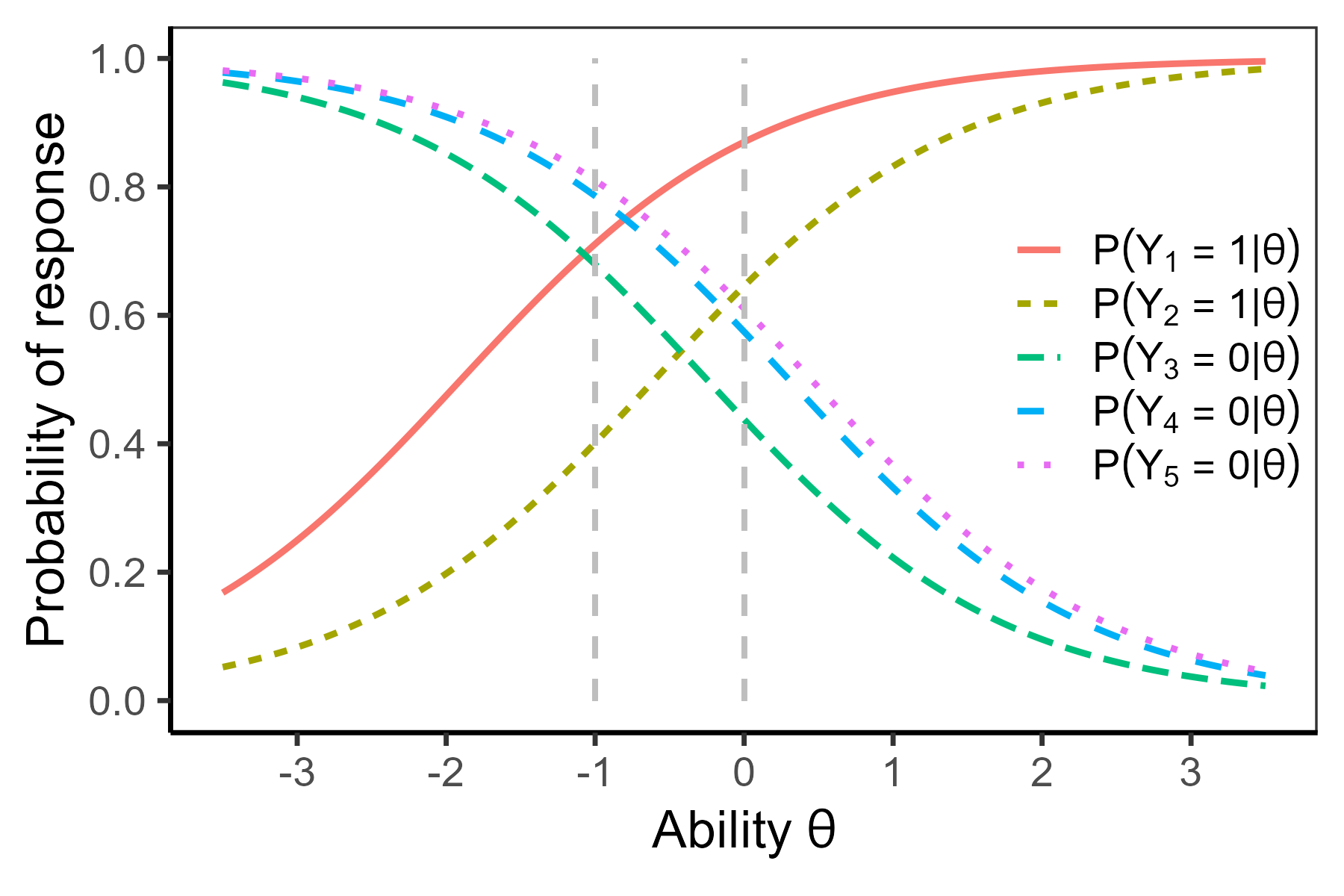
To find answers to the first two questions, we need to calculate the probability for each response in the pattern. Then, using the assumption of conditional independence, the probability of the response pattern 11000 is calculated as the product of probabilities for individual responses in the pattern. For the average respondent (\(\theta_p = 0\)), the probability of the correct answer to the first item with difficulty \(b_1 = -1.9\) is \[ \Pr(Y_{p1} = 1|\theta_p = 0) = \frac{\exp(\theta_p - b_1)}{1 + \exp(\theta_p - b_1)} = \frac{\exp(0 - (-1.9))}{1 + \exp(0 - (-1.9))} = 0.87 \] and it is \(0.65\) for the second item, whereas the probability of answering the last question incorrectly is \[ \Pr(Y_{p5} = 0|\theta_p = 0) = 1 - \frac{\exp(\theta_p - b_5)}{1 + \exp(\theta_p - b_5)} = 1 - \frac{\exp(0 - 0.45)}{1 + \exp(0 - 0.45)} = 0.61 \] and \(0.44\) and \(0.57\) for items 3 and 4, respectively.
Using the assumption of conditional independence, the likelihood (probability) of an average student providing a response pattern 11000 is \[ \begin{aligned} L(\theta_p = 0) =&\ \Pr(\boldsymbol{Y}_p = 11000|\theta_p = 0) = \prod_{i = 1}^5 \Pr(Y_{pi} = y_{pi}|\theta_p = 0) \\ =& \ \frac{\exp(1.9)}{1 + \exp(1.9)} \cdot \frac{\exp(0.6)}{1 + \exp(0.6)} \cdot \left(1 - \frac{\exp(0.25)}{1 + \exp(0.25)}\right) \\ & \ \cdot \left(1 - \frac{\exp(-0.3)}{1 + \exp(-0.3)}\right) \cdot \left(1 - \frac{\exp(-0.45)}{1 + \exp(-0.45)}\right) \\ =& \ 0.87 \cdot 0.65 \cdot 0.44 \cdot 0.57 \cdot 0.61 = 0.086, \end{aligned} \] whereas for a respondent with ability 1 SD below average \((\theta_p = -1)\), the likelihood to provide this response pattern is somewhat higher \[ L(\theta_p = -1) = \Pr(\boldsymbol{Y}_p = 11000|\theta_p = -1) = 0.71 \cdot 0.40 \cdot 0.68 \cdot 0.79 \cdot 0.81 = 0.123; \] also see Figure 7.5.
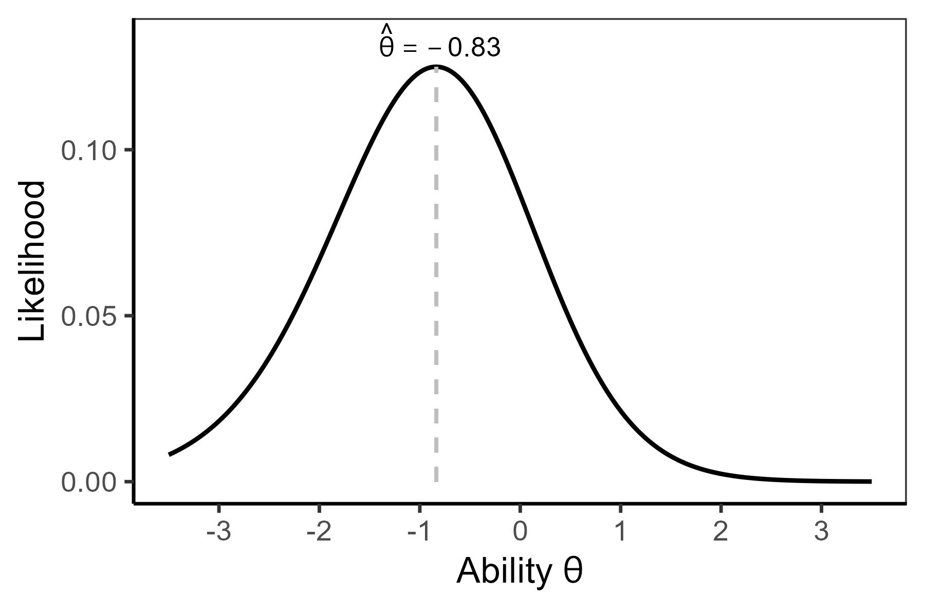
To answer the last question, and to find the ML estimate, the algorithm looks for the maximum of the likelihood as a function of \(\theta_p\) \[ \begin{aligned} L(\theta_p) =&\ \Pr(\boldsymbol{Y}_p = 11000|\theta_p) = \pi_1 \cdot \pi_2 \cdot (1 - \pi_3) \cdot (1 - \pi_4) \cdot (1 - \pi_5) \\ =&\ \frac{\exp(\theta_p + 1.9)}{1 + \exp(\theta_p + 1.9)} \cdot \frac{\exp(\theta_p + 0.6)}{1 + \exp(\theta_p + 0.6)} \cdot \left(1 - \frac{\exp(\theta_p + 0.25)}{1 + \exp(\theta_p + 0.25)}\right) \\ &\ \cdot \left(1 - \frac{\exp(\theta_p - 0.3)}{1 + \exp(\theta_p - 0.3)}\right) \cdot \left(1 - \frac{\exp(\theta_p - 0.45)}{1 + \exp(\theta_p - 0.45)}\right) \end{aligned} \] The shape of this likelihood function is provided in Figure 7.6 (a). The maximum likelihood appears to be obtained for an ability slightly above \(-1\).
The likelihood may be difficult to maximize, partly because it is a product of probabilities and with more items may reach values very close to zero. For this reason, it is easier to maximize the log-likelihood function Equation 7.9, which is more convenient to handle and which reaches its maximum at the same ability level as the likelihood function, in this case at \(\theta = - 0.83\), also see Figure 7.6 (b). \[ \begin{aligned} l(\theta_p) =&\ \log\left(\Pr(\boldsymbol{Y}_p = 11000|\theta_p)\right)\\ =&\ \log\left(\frac{\exp(\theta_p + 1.9)}{1 + \exp(\theta_p + 1.9)}\right) + \log\left(\frac{\exp(\theta_p + 0.6)}{1 + \exp(\theta_p + 0.6)}\right) \\ &\ + \log\left(1 - \frac{\exp(\theta_p + 0.25)}{1 + \exp(\theta_p + 0.25)}\right) + \log\left(1 - \frac{\exp(\theta_p - 0.3)}{1 + \exp(\theta_p - 0.3)}\right) \\ &\ + \log\left(1 - \frac{\exp(\theta_p - 0.45)}{1 + \exp(\theta_p - 0.45)}\right). \end{aligned} \]
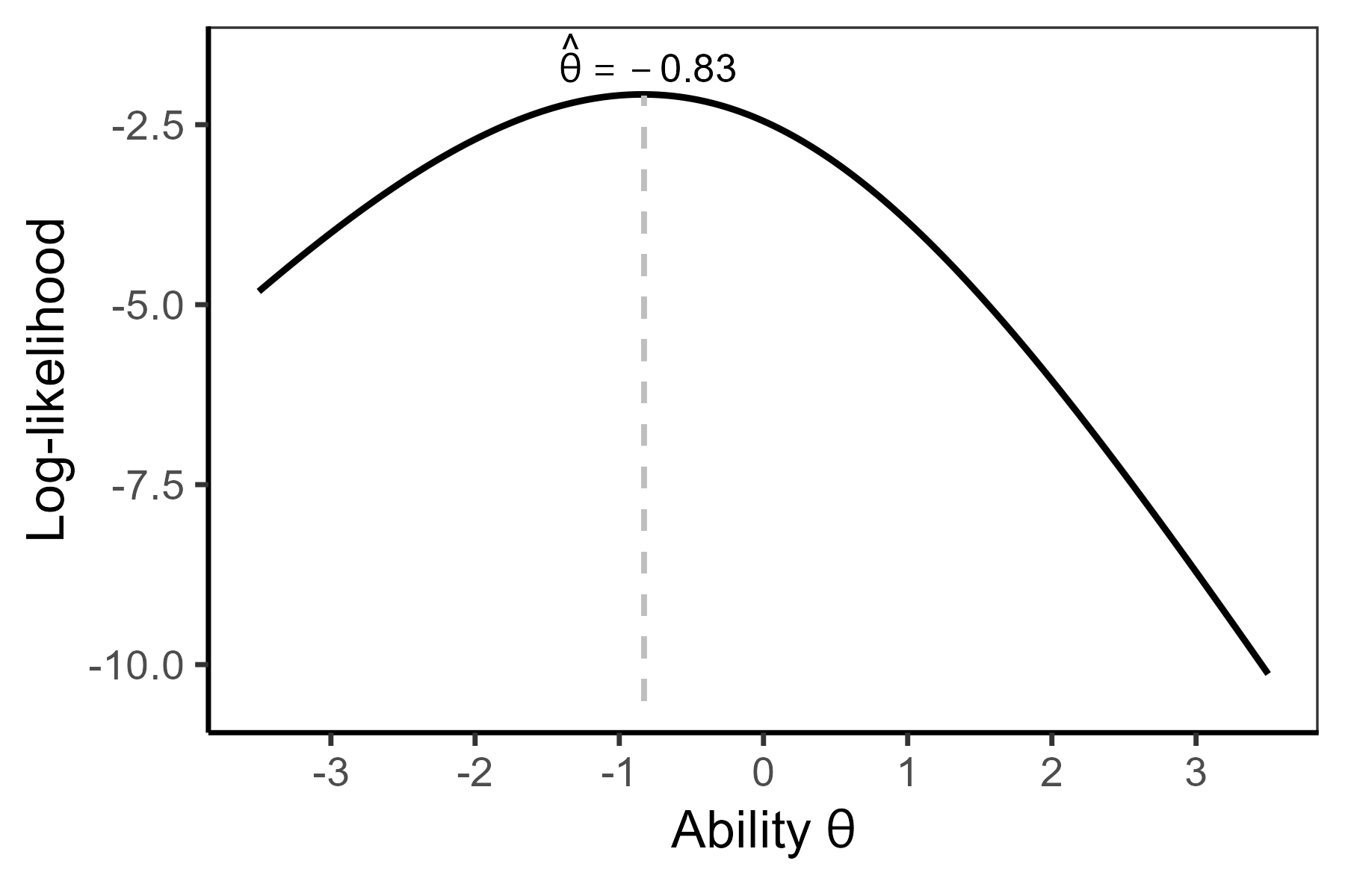
The maximization of the log-likelihood involves the calculation of partial derivatives and solving corresponding likelihood equations, in which the derivatives of the log-likelihood function with respect to estimated parameter are set at equal to zero. These equations often do not have a solution of closed forms; therefore, numerical approaches are needed. A popular method is the Newton-Raphson algorithm, which looks for a zero derivative of log-likelihood Equation 7.9, \(l'(\theta)\), i.e., the (local) maximum, using the second derivative of log-likelihood \(l''(\theta)\) to find it quickly. In each step of the algorithm, the new estimate is found as \[ \hat{\theta}_{\textrm{new}} = \hat{\theta}_{\textrm{old}} - \frac{l'(\hat{\theta}_{\textrm{old}})}{l''(\hat{\theta}_{\textrm{old}})}. \] Once the algorithm converges (i.e., the difference between \(\hat{\theta}_{\textrm{old}}\) and \(\hat{\theta}_{\textrm{new}}\) is small enough), the \(\hat{\theta}_{\textrm{new}}\) in the final step of the Newton-Raphson algorithm is used as the ability estimate. The derivatives can be further used for the estimation of item information and the standard error of the ability estimate, see Section 7.3.6.
Example: Estimating item parameters in the JML algorithm. In the next step of the JML algorithm, the person parameters would be considered fixed and the item parameters would be estimated given the response pattern of all 20 respondents for a given item. This problem was already addressed in Section 6.5, where respondent ability was considered observed and readily available.
In the 1PL model, the algorithm would determine the ML estimate as the most likely difficulty parameter for the item to provide this given response pattern. If the underlying model was a 2PL model, the likelihood function would be 2-dimensional. The 3PL and 4PL models bring, besides an even higher dimensionality of the likelihood function, further issues including the need for the restriction of the pseudo-guessing and inattention parameters \(c_i\) and \(d_i\) to interval \([0, 1]\). For very easy or very difficult items, the likelihood function may have multiple local maxima, and it may be especially hard to estimate the asymptote parameters unless enough respondents have very low or very high ability levels respectively.
The JML estimates suffer from being inconsistent (Andersen, 1970). This, in terms of IRT models, means that no matter how many individuals are included in the sample, the estimates for the item parameters may still be biased.
7.3.3 Conditional maximum likelihood
For the Rasch/1PL model, Andersen (1970) suggested conditioning the likelihood by the total score \(X_p = Y_{p\bullet} = \sum_{i = 1}^m Y_{pi}\), as an alternative ML method for the estimation. In this CML approach, we use the fact that in the Rasch model, the total score \(X_p\) is the minimal sufficient statistic for the person abilities. In other words the conditional likelihood does not depend on ability \(\theta\):
\[ \Pr(\boldsymbol{Y} = \boldsymbol{y}|\theta, \boldsymbol{b}, \boldsymbol{Y}_{p\bullet} = r_p) = \frac{\exp\left(-\sum_{i = 1}^m y_{pi} b_i\right)}{\sum_{\left\{\boldsymbol{x}: \sum_{i = 1}^m x_i = r_p\right\}} \exp\left(-\sum_{i = 1}^m x_{i} b_i\right)}, \tag{7.10}\]
considering all possible response patterns \(\boldsymbol{x}\) which lead to the same total score, \(\sum_{i = 1}^m x_i = r_p\), as the observed response pattern. The conditional likelihood can then be maximized with respect to the item difficulty parameters \(\boldsymbol{b} = (b_1, \dots, b_m)\).
This method can only be used to fit Rasch-type models, i.e., besides the Rasch and the 1PL model, also their polytomous extensions. More complex IRT models, including the 2PL and 3PL IRT models, do not have a simple sufficient statistic for an ability estimate.
As was the case in the JML algorithm, the model here is also not identified and further constraints need to be placed on the item parameters. Usually, the sum of item difficulty parameters is restricted at zero, or the first item difficulty parameter is restricted at zero.
7.3.4 Marginal maximum likelihood
The method of the MML places a prior assumption on the distribution of the ability \(\theta\). It is typical to assume that ability follows a normal distribution; however, technically, it is possible to use any (reasonable) distribution \(g(\theta)\). Since no assumption on the ability distribution was set in the case of JML, in this instance the MML method is more restrictive. Marginal likelihood is calculated as the weighted average across the ability spectrum, where the ability distribution \(g(\theta)\) serves as a weight:
\[ L(\boldsymbol{\xi}) = \Pr(\boldsymbol{Y} = \boldsymbol{y}|\boldsymbol{\xi}) = \int_{-\infty}^\infty \Pr(\boldsymbol{Y} = \boldsymbol{y}|\theta, \boldsymbol{\xi}) \cdot g(\theta) \, \mathrm{d}\theta. \tag{7.11}\]
The resulting marginal likelihood function Equation 7.11 does not depend on ability \(\theta\). Rather, the MML specifies the unconditional, marginalized probability that a randomly selected respondent from the population with a distribution of latent abilities \(g(\theta)\) provides response vector \(\boldsymbol{Y}\). To obtain the parameter estimates, the MML Equation 7.11 is maximized with respect to item parameter(s) \(\boldsymbol{\xi}\).
The indeterminacy of the item estimates is again solved by additional constraints. These are placed either on the item parameters or on the parameters (mean and standard deviation) of the prior distribution \(g(\theta)\), most often yielding the assumption of standard normal distribution.
Integration in likelihood equations based on Equation 7.11 is typically solved using a numerical algorithm, such as the Gauss-Hermite quadrature (numerical integration), which can be understood as a weighted sum: At each theta interval, the likelihood of a response pattern rectangle is weighted by that rectangle’s probability of being observed.
The MML approach, using a Fisher scoring method, involves calculation of inverse matrices which is computationally demanding in a high number of items. A computationally tractable alternative involves using an iterative algorithm, termed the EM algorithm, in the context of the IRT models proposed in Bock & Aitkin (1981). The EM algorithm is a general numerical method for the maximization of a likelihood which depends upon unobserved latent variables (Dempster et al., 1977). The algorithm consists of two steps:
- In the E-step (expectation step), the expected value of the log-likelihood of the parameters is calculated, with the expectation taken over the conditional distribution of the unobserved latent variables \(\theta\), given the observed data (item responses).
- In the M-step (maximization step) this resulting likelihood function is maximized with respect to the parameters.
7.3.4.1 Estimation of person abilities in MML
In addition to estimation of the item parameters, estimation of the respondent ability is important. This can be done by several methods, based upon either ML or Bayesian approaches.
Assuming that the item parameters are known, the ability parameter \(\theta\) may be estimated from item responses by using the ML method. This was already described in Section 7.3.2, including a demonstration of a practical example. Specifically, for a single respondent with a response pattern \(\boldsymbol{y} = (y_1, \dots, y_m)\), the ML estimate \(\hat{\theta}\) of \(\theta\) is obtained by maximizing the likelihood function \[ L(\theta, \boldsymbol{y}) = \Pr(\boldsymbol{Y} = \boldsymbol{y}|\theta, \boldsymbol{\xi}) = \prod_{i = 1}^m \pi_{i}^{y_{i}} \left(1 - \pi_{i}\right)^{1 - y_{i}}, \] where \(\boldsymbol{\xi}\) is a set of item parameters.
A weakness of the ML method is the fact that the ability estimate reaches infinity values for respondents with all correct or all incorrect answers. In practice, such respondents will then need to be removed. An alternative is the weighted likelihood which can also provide less biased estimation (Warm, 1989).
A special case of the weighted ML estimate is the Bayesian estimate of ability, which is based upon the posterior distribution of ability \[ h(\theta, \boldsymbol{y}) = C g(\theta) L(\theta, \boldsymbol{y}), \] with \(L(\theta, \boldsymbol{y}\)) being the likelihood function, \(g(\theta)\) being a prior density of random variable \(\theta\) which describes our prior beliefs of the ability distribution, and \(C = \frac{1}{\int g(\theta) L(\theta, \boldsymbol{y}) \, \mathrm{d}\theta}\) being a constant set to obtain density, i.e., the scaling parameter.
The Bayes modal estimator, also termed maximum a posteriori (MAP) or empirical Bayes (EB) estimator, uses the mode of the posterior distribution to estimate the latent ability. As another option, the expected a posteriori (EAP) estimator uses the expected value of the posterior distribution.
Let’s now take a closer look at the precision of the ML ability estimate \(\hat{\theta}\). Under some regularity conditions, which may be shown to hold for joint distributions of logistic models, the ML estimate \(\hat{\theta}\) is consistent (i.e., converges in probability to the true value \(\theta_0\)) and is asymptotically normally distributed with a variance equal to an inverse of the so-called Fisher information \(\mathrm{I}(\theta_0)\): \[ \sqrt{m}(\hat{\theta} - \theta_0) \xrightarrow[]{\mathcal{D}} \mathcal{N} (0, \mathrm{I}^{-1}(\theta_0)). \]
The observed Fisher information is defined as the negative value of the second derivative of the log-likelihood Equation 7.9 with respect to \(\theta\),
\[ \mathrm{I}(\theta, Y) = -\frac{\partial^2 l(\theta)}{\partial \theta^2}. \tag{7.12}\]
The Fisher information is then defined as the expected value of the observed Fisher information, \(\mathrm{I}(\theta) = \text{E} \, \mathrm{I}(\theta, Y)\). For each level of ability, the inverse of the test information provides a standard error of the ability estimate
\[ \text{SE}(\hat{\theta}) = \sqrt{\mathrm{I}^{-1}(\hat{\theta})}, \tag{7.13}\]
and a \(95\%\) confidence interval for the ability estimate in form \[ (\hat{\theta} - 1.96 \cdot \sqrt{\mathrm{I}^{-1}(\hat{\theta})}, \hat{\theta} + 1.96 \cdot \sqrt{\mathrm{I}^{-1}(\hat{\theta})}). \]
Note, however, that the standard error of the ability estimate Equation 7.13 relies on the assumption of a correctly specified IRT model, and that the approximation is only valid for a sufficiently large number of items (Ippel & Magis, 2020). As another option, re-sampling methods may be used to obtain individual standard errors.
7.3.5 Bayesian IRT models
The Bayesian approach to estimation in IRT models (Richard J. Patz & Junker, 1999a; Richard J. Patz & Junker, 1999b) is analogous to Bayesian estimate of ability discussed within the MML. Along with the ability parameters, it also sets a prior distribution on the item parameters. Except for the simple cases of so-called conjugate priors, which give closed-forms of posterior distributions, sampling algorithms such as MCMC methods need to be used.
7.3.6 Item and test information
An important characteristic of the test and of its individual items describes how much information is provided by them in estimating ability of a certain level. Formulae Equation 7.13 and Equation 7.12 suggest that the precision of the ability estimate depends on Fisher information, which is calculated using derivatives of the log-likelihood.
This characteristic can be used to describe a test and its items. For a given ability level, the test information function (TIF) \(\mathrm{I}(\theta)\) is related to the inverse of the standard error of the measurement, see Equation 4.6. Here, the standard error is provided for each ability level, \(\text{SE}(\theta)\). It can also be used to describe test reliability \(\rho_{X}(\theta)\) for a given ability level also considering the variance of the latent trait \(\sigma^2\), which is often assumed to be fixed at 1:
\[ \text{SE}(\theta) = \frac{1}{\sqrt{\mathrm{I}(\theta)}} = \sigma \sqrt{(1 - \rho_{X}(\theta))}. \tag{7.14}\]
Intuitively, the TIF will be lowest for low and high ability levels, for which there are not enough items of appropriate difficulty. Considering individual items, intuitively, an item provides the most information for those ability levels near to item difficulty, where the slope of the ICC is the highest: For these abilities the item is most precisely able to distinguish between respondent ability levels because for a given difference in ability, the difference in the probability of a correct answer is the largest. This intuition can be formalized by defining item information.
Considering the local independence assumed in the IRT models and the form of the log-likelihood function Equation 7.9, it is possible to split the information into contributions from the individual items. Let us define \(l_i(\theta)\) as the contribution of item \(i\) to the log-likelihood Equation 7.9 \[ l_i(\theta) = Y_i \log \pi_i (\theta) + (1 - Y_i) \log (1 - \pi_i(\theta)). \] where \(\pi_i(\theta)\) is the item probability function for a given IRT model.
The observed item information function can then be defined, similar to the observed information Equation 7.12, as the negative value of the second partial derivative of the item contribution to the log-likelihood with respect to \(\theta\). The form of the observed item information function is then
\[ \begin{aligned} \mathrm{I}_i(\theta, Y_i) &= -\frac{\partial^2 l_i(\theta)}{\partial \theta^2} \\ &= Y_i \, \frac{(\pi_i^{'}(\theta))^2 - \pi_i(\theta)\pi_i^{''}(\theta)}{\pi_i^2(\theta)} + (1 - Y_i) \, \frac{\pi_i^{''}(\theta)(1 - \pi_i(\theta)) + (\pi_i^{'}(\theta))^2}{(1 - \pi_i(\theta))^2}. \end{aligned} \tag{7.15}\]
The item information function (IIF) is defined as the expected value of the observed item information function Equation 7.15, and can be expressed as
\[ \mathrm{I}_i(\theta) = \text{E} \, \mathrm{I}_i(\theta, Y_i) = \frac{(\pi_i^{'}(\theta))^2}{\pi_i(\theta) (1 - \pi_i(\theta))}. \tag{7.16}\]
Let us first consider the 2PL model Equation 7.3. The IIF Equation 7.16 has then the form \[ \mathrm{I}_i(\theta) = \frac{(\pi_i^{'}(\theta))^2}{\pi_i(\theta) (1 - \pi_i(\theta))} = \frac{\left[a_i \pi_i(\theta) (1 - \pi_i(\theta))\right]^2}{\pi_i(\theta) (1 - \pi_i(\theta))} = a_i^2 \pi_i(\theta) (1 - \pi_i(\theta)). \] For the Rasch model, i.e., \(a_{i} = 1\), the IIF is equal to \(\mathrm{I}_i(\theta) = \pi_{i}(\theta) (1 - \pi_{i}(\theta))\).
More generally, when considering the 4PL IRT model Equation 7.6, the IIF Equation 7.16 is of the following form:
\[ \mathrm{I}_i(\theta) = a_{i}^{2}{\frac {(\pi_{i}(\theta) - c_{i})^{2}}{(d_i - c_{i})^{2}}}{\frac {(d_i - \pi_{i}(\theta))^2}{\pi_{i}(\theta)(1 - \pi_{i}(\theta))}}, \tag{7.17}\]
see Exercise 7.3. The formula Equation 7.17 for the 3PL IRT model Equation 7.5 simplifies into: \[ \mathrm{I}_i(\theta) = a_{i}^{2}\frac{(\pi_{i}(\theta) - c_{i})^{2}}{(1 - c_{i})^{2}}{\frac{(1 - \pi_{i}(\theta))}{\pi_{i}(\theta)}}. \]
Let us now return to the test information, \(\mathrm{I}(\theta)\), which is describing the amount of information provided by all item responses on a test for a given ability level. Considering the form Equation 7.9, the TIF is calculated as the sum of the IIFs for individual items:
\[ \mathrm{I}(\theta) = \sum_{i = 1}^m \mathrm{I}_i(\theta). \tag{7.18}\]
The graphical representations of IIF defined by Equation 7.16 and of TIF defined by Equation 7.18 are termed item information curve (IIC) and test information curve (TIC), respectively. When displayed, these curves may provide guidance on usefulness of the test and of a given item for different ability levels.
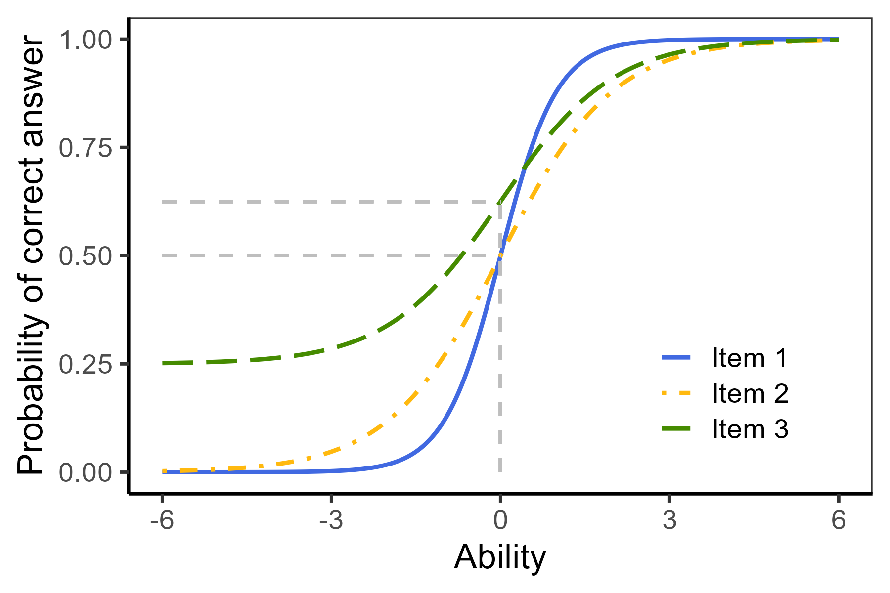
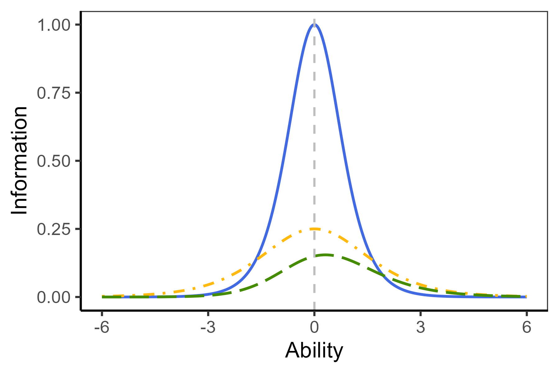
Note that those items with a high discrimination also provide high information, but on a rather small interval of ability levels which are close to an item difficulty in 1PL and 2PL models (see item 1 in Figure 7.7). Items with a lower discrimination have a lower maximal information, which may, however, be higher for those ability levels further from the item difficulty than in higher discriminating items of the same difficulty (see item 2 in Figure 7.7). From the form of IIF Equation 7.17, it is also apparent that for the 3PL and 4PL model, the item information is not necessarily the highest at an ability level equal to the item difficulty, as was the case in the 2PL model (see item 3 in Figure 7.7).
7.3.7 Model selection and model fit
Model selection methods and criteria described in Section 6.6 may be used to select between competing models and to assess model fit. Decision between the two nested models may be performed with the LRT Equation 2.29. This test is appropriate for comparison between 1PL and 2PL IRT models; however, caution is needed as was discussed in Section 6.6.1: For comparison between the 2PL, 3PL, and 4PL models, the LRT is not appropriate, because the submodels are defined by restricting the guessing parameter \(c_i\) to 0, and/or the inattention parameter \(d_i\) to 1, which are the boundary values; thus the assumptions for asymptotic properties of the test are violated.
Comparison of the competing models may also be done using the AIC Equation 2.30 or BIC Equation 2.31. No statistical inference is involved; the comparison is thus appropriate even for 2PL, 3PL, and 4PL models. Lower values signal the better performing model.
Alternatively, considering the categorical nature of the data, the model fit may be evaluated using goodness-of-fit tests based on contingency tables (Agresti, 2002). The general idea of the Pearson’s goodness-of-fit \(\chi^2\) test is as follows: For the response pattern \(\boldsymbol{y} = (y_1, \dots, y_m)\), let the \(O_{\boldsymbol{y}}\) be the observed number of respondents with this response pattern, and let \(E_{\boldsymbol{y}}\) be the expected number of respondents according to the tested model. The Pearson’s \(\chi^2\) test uses the sum of squared differences between observed and expected frequencies divided by the expectation: \[ T = \sum_{\boldsymbol{y}} \frac{\left(O_{\boldsymbol{y}} - E_{\boldsymbol{y}}\right)^2}{E_{\boldsymbol{y}}}. \] When the model holds, the \(T\) statistic approximately follows a \(\chi^2\) distribution Equation C.5.
The problem with this general approach is that with a higher number of items, some response patterns will rarely occur, and the frequencies for individual response patterns will be low, thus violating assumptions of the test. For this reason, in practice and in the context of the IRT models, instead of using individual response patterns, the response patterns are combined, e.g., for predefined ability groups. Fit indices analogous to those described in Section 3.4.5 may also be implemented. For more details on available goodness-of-fit tests and fit measures for IRT models, see Debelak et al. (2022, 4).
7.4 IRT models in R
In this section, we will introduce several R packages for fitting IRT models. We will start with the mirt package, which is the most comprehensive one. We will then present the ltm and eRm packages, which are more focused on specific models. We will also mention the TAM, ShinyItemAnalysis, lme4, and brms packages.
7.4.1 The mirt package
The mirt package (Chalmers, 2012) offers a comprehensive framework for fitting IRT models. The function mirt() can be used to fit a wide range of IRT models, including the 1PL, 2PL, 3PL, and 4PL models. The MML method using the EM algorithm is used for model estimation.
Rasch/1PL model. To fit the Rasch/1PL IRT model Equation 7.1 to the HCI dataset, we specify the itemtype = "Rasch" argument:
library(mirt)
fit_rasch_mirt <- mirt(HCI[, 1:20], model = 1, itemtype = "Rasch")
coef(fit_rasch_mirt, IRTpars = TRUE, simplify = TRUE)$items
##         a       b  g  u
## Item 1  1 -0.9769  0  1
## Item 2  1 -1.2802  0  1
## Item 3  1 -1.9397  0  1
## ...
## Item 20 1 -1.0640  0  1
The column a denotes item discrimination which is constrained to 1, column b then provides item difficulty estimates, and columns g and u pertain to the pseudo-guessing and inattention parameters (fixed at 0 and 1, respectively).
1PL IRT model. To fit the 1PL IRT model with common but unconstrained discrimination, we specify itemtype = "2PL" and constrain the discrimination parameter to be the same for all items. We then set IRTpars = TRUE to display IRT parametrization with common discrimination \(a = 0.86\):
fit_1PL_mirt <- mirt(HCI[, 1:20], model = 1, itemtype = "2PL",
                     constrain = list((1:20) + seq(0, (20 - 1) * 3, 3)))
coef(fit_1PL_mirt, IRTpars = TRUE, simplify = TRUE)$items
##           a       b  g  u
## Item 1  0.86 -1.0046  0  1
## Item 2  0.86 -1.3053  0  1
## ...
## Item 20 0.86 -1.0924  0  1
2PL IRT model. To fit the 2PL IRT model Equation 7.3, we simply change the item type to "2PL" and remove the constraint on discrimination. The 2PL model provides a discrimination estimate specific to each item:
fit_2PL_mirt <- mirt(HCI[, 1:20], model = 1, itemtype = "2PL")
coef(fit_2PL_mirt, IRTpars = TRUE, simplify = TRUE)$items
##            a       b  g  u
## Item 1  0.8509 -1.1457  0  1
## Item 2  0.7167 -1.7229  0  1
## Item 3  1.5745 -1.5262  0  1
## ...
## Item 20 0.9886 -1.1624  0  1
3PL IRT model. To fit the 3PL IRT model Equation 7.5, we use itemtype = "3PL":
fit_3PL_mirt <- mirt(HCI[, 1:20], model = 1, itemtype = "3PL")
coef(fit_3PL_mirt, IRTpars = TRUE, simplify = TRUE)$items
##             a       b      g  u
## Item 1  0.6706 -1.7684 0.1403  1
## Item 2  0.7211 -1.8277 0.0355  1
## ...
## Item 20 0.8076 -1.6098 0.1321  1
4PL IRT model. To fit the 4PL IRT model Equation 7.6, we use itemtype = "4PL":
fit_4PL_mirt <- mirt(HCI[, 1:20], model = 1, itemtype = "4PL")
coef(fit_4PL_mirt, IRTpars = TRUE, simplify = TRUE)$items
##             a       b      g      u
## Item 1  0.7014 -1.7289 0.1418 0.9957
## ...
## Item 20 0.7909 -1.6666 0.1337 0.9952
ICCs, IICs, and TIC. Once the IRT model has been fitted, ICCs may be plotted with the itemplot() function. In Figure 7.8, we display the ICCs for the 2PL IRT model on the HCI dataset.
itemplot(fit_2PL_mirt, item = 1, type = "trace")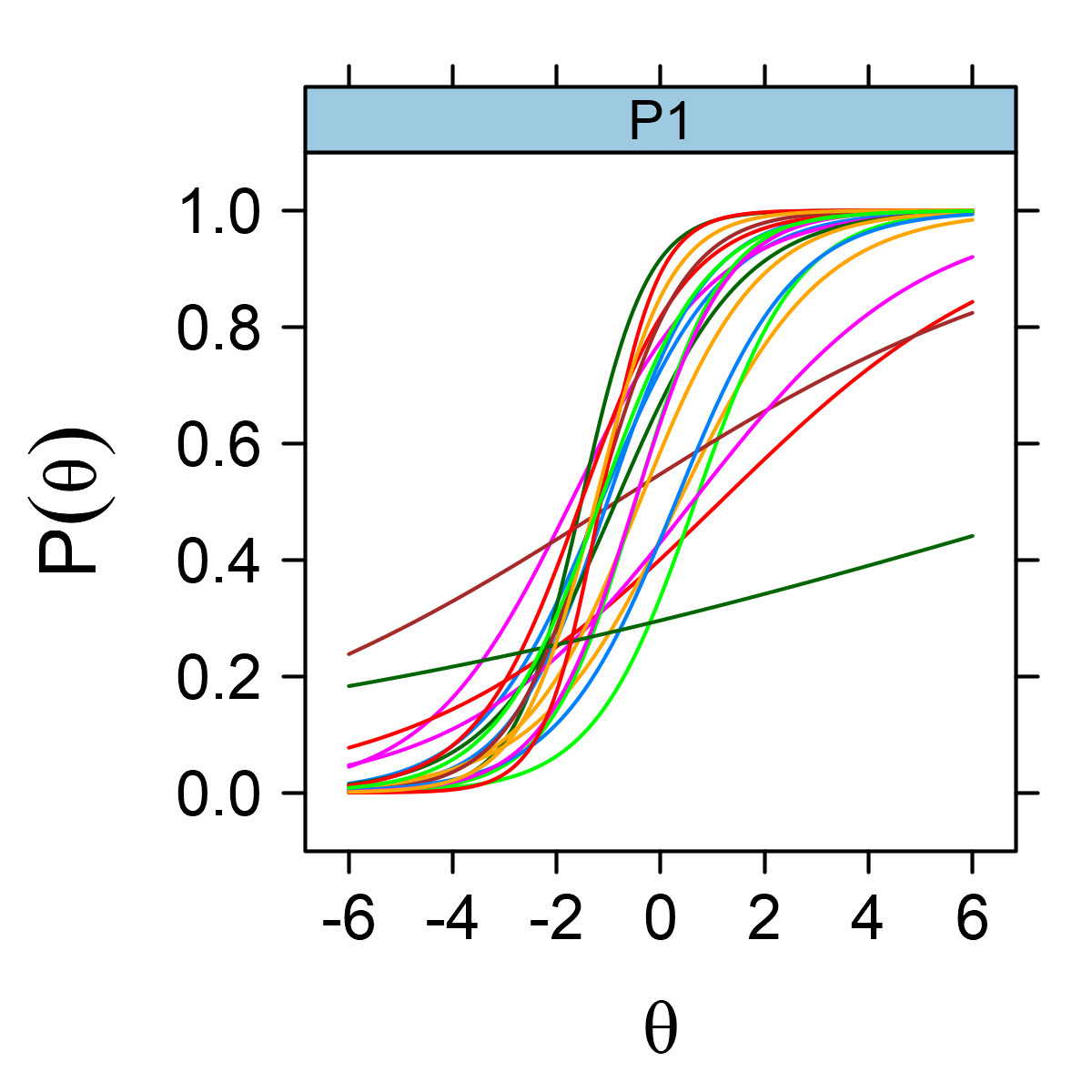
mirt package on the HCI dataset.
The IICs can be plotted using the argument type = "info" within the itemplot() function (Figure 7.9):
itemplot(fit_2PL_mirt, item = 1, type = "info")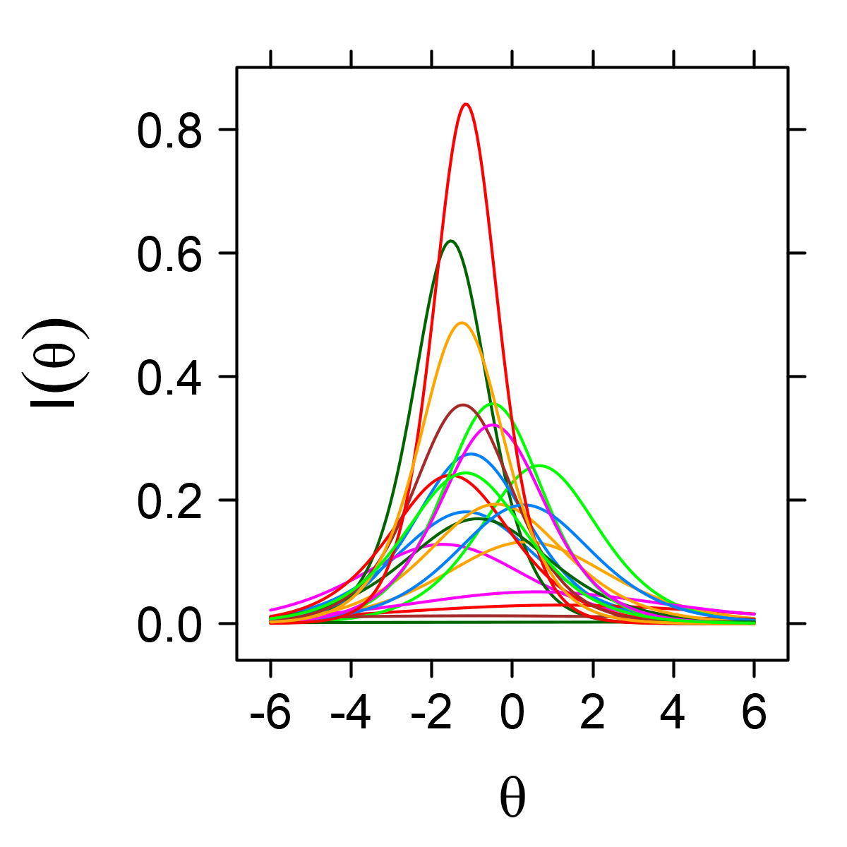
mirt package on the HCI dataset.
The TIC, or its counterpart, the standard error of measurement as a function of ability, can be obtained from the plot() method (Figure 7.10).
plot(fit_2PL_mirt, type = "info")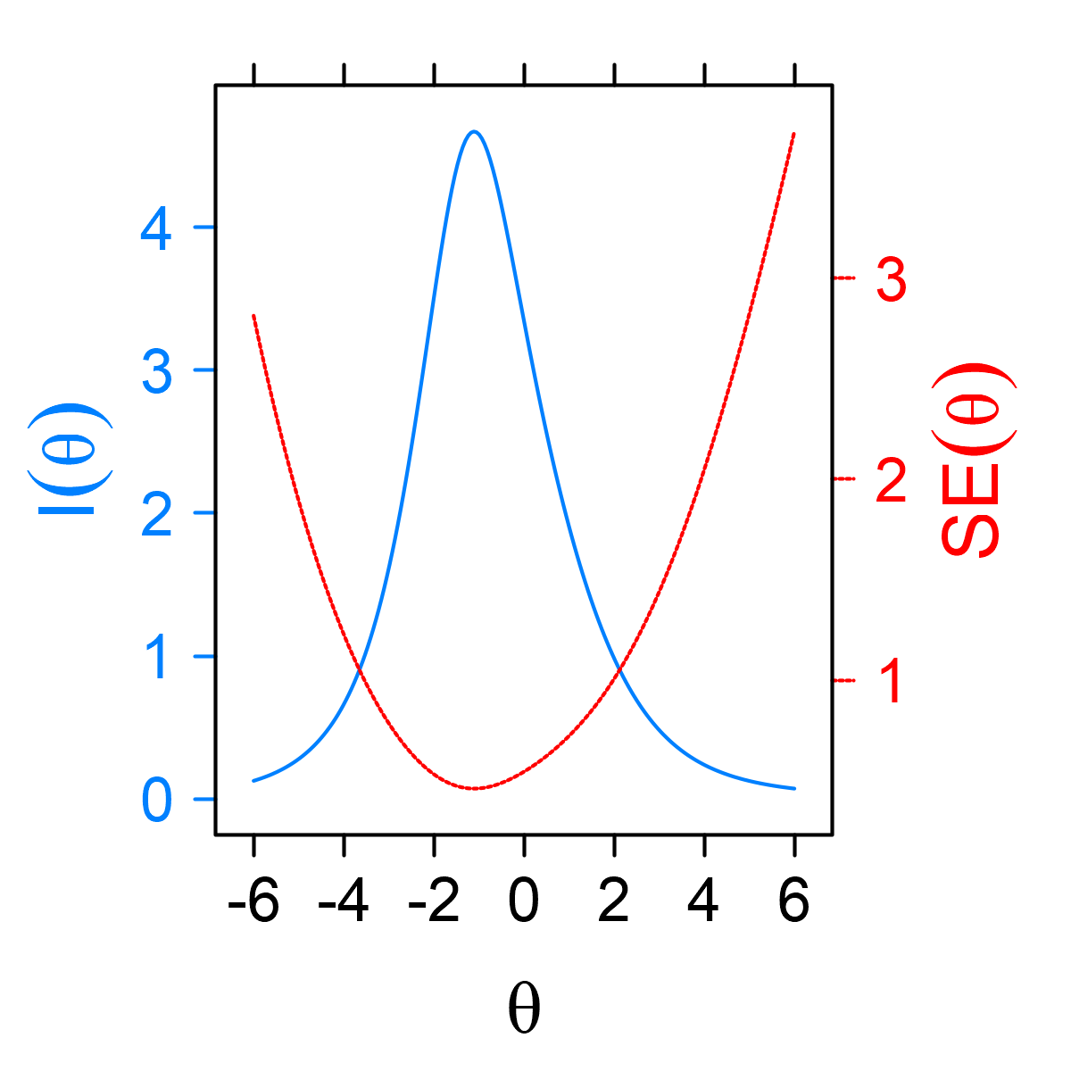
mirt package on the HCI dataset.
Estimating latent abilities. Using the fscores() function, latent abilities can be estimated with several methods, including expected a posteriori (EAP, the default method), maximum a posteriori (MAP), maximum likelihood (ML), or weighted likelihood (WLE). Values of item parameters are considered fixed.
fs_rasch <- fscores(fit_rasch_mirt)
head(fs_rasch)
##            F1
## [1,]  0.6832
## [2,]  1.4920
## [3,] -0.2373
## ...
Figure 7.11 presents the distribution of the estimated factor scores from the Rasch model. These scores indeed offer an approximation of the assumed standard normal distribution.
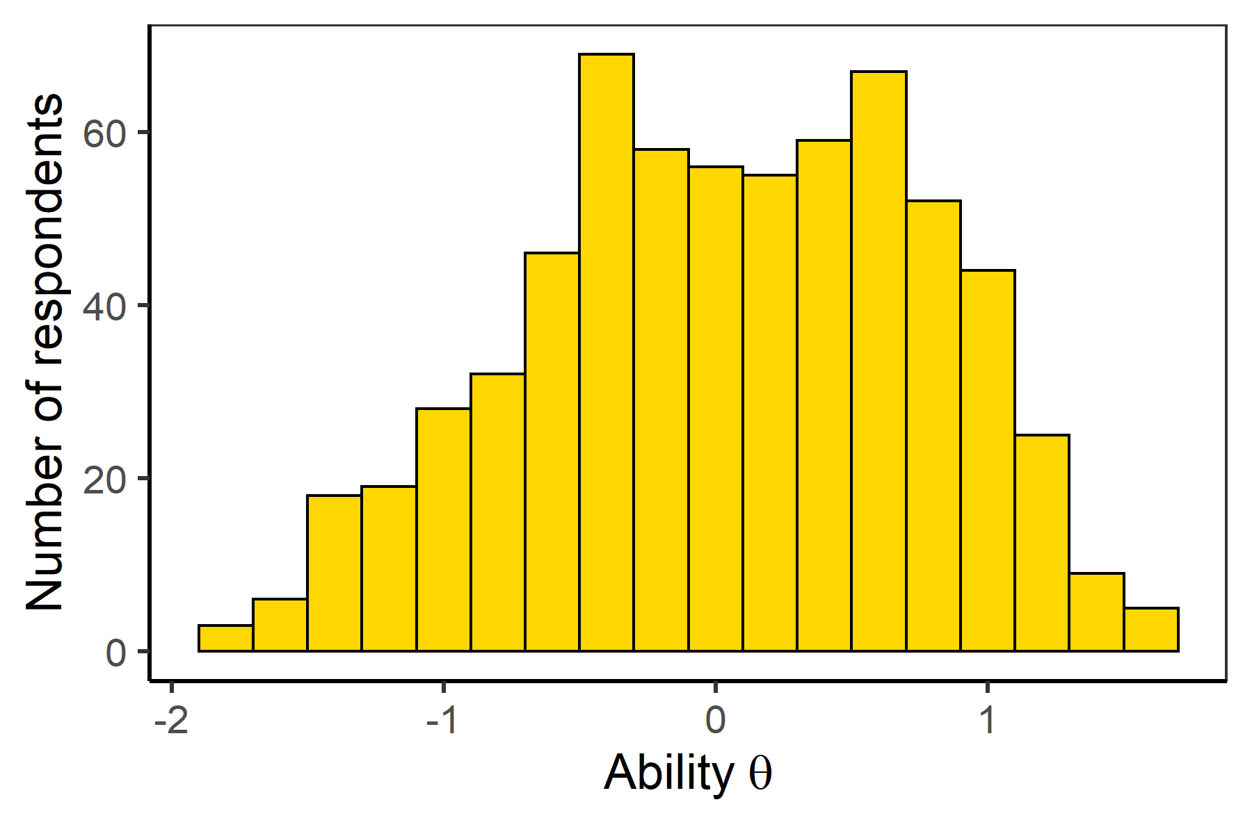
HCI dataset.
The latent abilities from the Rasch model are also related to the standardized total score (Figure 7.12), obtained as \(Z_p = (X_p - \bar{X})/s_X\). This connection was discussed in Test Score Function (see also Equation 7.10).

HCI dataset with the Rasch model.
ICCs for the Rasch model. The Rasch model ICCs for the HCI dataset are displayed in Figure 7.13. Item 3 was the easiest and Item 17 the most difficult.
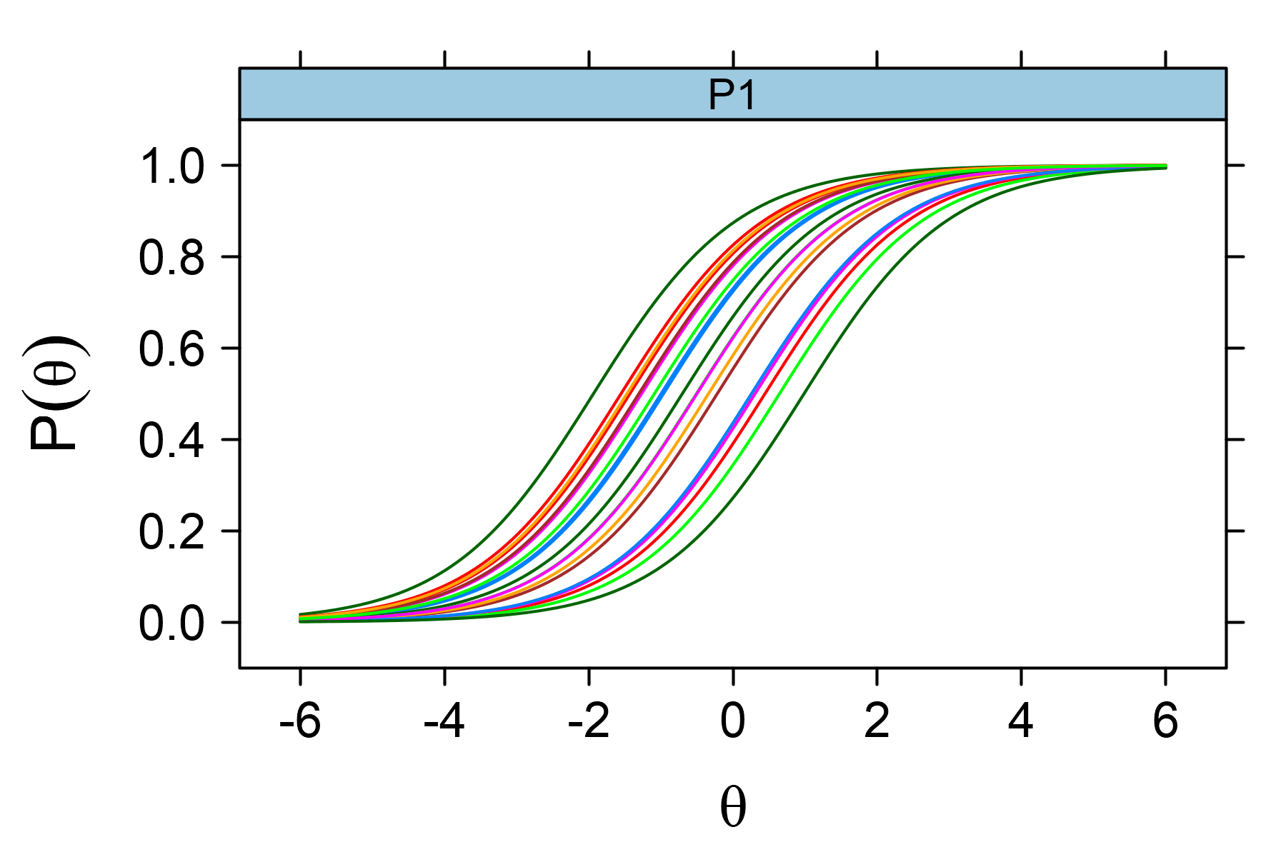
mirt package on the HCI dataset.
7.4.2 The ltm package
The ltm package (Rizopoulos, 2006) offers functions for the estimation of the Rasch/1PL, 2PL, and 3PL IRT models using the MML method.
Rasch model. To fit the Rasch model, we use the rasch() function. The parametrization with a common discrimination \(a\) is used:
library(ltm)
fit_rasch_ltm <- rasch(HCI[, 1:20])
coef(fit_rasch_ltm)
##         Dffclt Dscrmn
## Item 1  -0.992 0.8266
## Item 2  -1.299 0.8266
## ...
## Item 20 -1.080 0.8266
To verify that the difficulty parameters are similar to those from the mirt package, they can be obtained by dividing the difficulty estimate by the discrimination estimate \(b_i/a = -0.992/0.8266 = -1.20\), which is close to the difficulty of item 1 from the mirt package, and exactly equal to it when fixing \(a = 1\) in the constrained Rasch model. The parametrization may alternatively be set to "Rasch" to receive parameters under \(a = 1\).
2PL model. The ltm() function fits the 2PL IRT model Equation 7.3 either in a unidimensional or two-dimensional form specified by factors z1 and z2 in the formula argument. Here we show only the unidimensional example:
fit_2PL_ltm <- ltm(HCI[, 1:20] ~ z1)
coef(fit_2PL_ltm)
##         Dffclt Dscrmn
## Item 1  -1.1459 0.8511
## Item 2  -1.7226 0.7167
## ...
## Item 20 -1.1617 0.9886
3PL model. In the ltm package, the 3PL IRT model Equation 7.5 can be fitted with the tpm() function.
fit_3PL_ltm <- tpm(data = HCI[, 1:20])
coef(fit_3PL_ltm)
##        Gussng  Dffclt Dscrmn
## Item 1  0.2983 -0.3177 1.0864
## Item 2  0.1785 -1.2092 0.7837
## ...
## Item 20 0.0678 -1.0653 0.9437
The item parameter estimates from the ltm package are once again very similar to those from the mirt package.
Estimating latent abilities. The factor.scores() function of the ltm package can be used to extract estimates of person abilities and their standard errors Equation 7.13. This function uses the MAP as a default option and allows for other methods by setting the argument method. By default, the function returns latent abilities for unique response patterns.
ltm::factor.scores(fit_rasch_ltm)
## Factor-Scores for observed response patterns:
##    Item 1 Item 2 ... Item 18 Item 19 Item 20 Obs   Exp     z1 se.z1
## 1       0      0 ...       1       1       0   1 0.002 -1.450 0.454
## 2       0      0 ...       0       0       0   1 0.017 -1.885 0.481
## ...
In the output, the response patterns present in the data are presented in rows and complemented by the estimated latent ability z1 and its standard error se.z1. For the first response pattern (0, 0, …, 1, 1, 0), the estimated latent ability is \(-1.450\) with a standard error \(0.454\).
To obtain the latent abilities of the respondents ordered as in data frame HCI, argument resp.patterns needs to be used to specify the response patterns of the respondents.
ltm::factor.scores(fit_rasch_ltm, resp.patterns = HCI[, 1:20])
## Factor-Scores for specified response patterns:
##    Item 1 Item 2 ... Item 18 Item 19 Item 20 Obs   Exp     z1 se.z1
## 1       1      1 ...       1       1       1   2 0.188  0.754 0.488
## 2       1      1 ...       1       1       1   3 0.991  1.578 0.570
## ...
Moreover, the argument resp.patterns may also be specified as a new response pattern.
ltm::factor.scores(fit_rasch_ltm,
                   resp.patterns = matrix(rep(c(1, 0), each = 10), nrow = 1))
## Factor-Scores for specified response patterns:
##    Item 1 Item 2 ... Item 18 Item 19 Item 20 Obs Exp     z1 se.z1
## 1       1      1 ...       0       0       0   0   0 -0.482 0.436
As an example, a respondent who answered the first 10 items correctly and the next 10 items incorrectly has an estimated ability of \(-0.48\) using the Rasch model.
7.4.3 The eRm package
The next option for fitting the IRT models is the RM() function of the eRm package. The eRm package implements the conditional maximum likelihood for parameter estimation. This limits the options to Rasch-type models, as it is not possible to estimate 2 or more parameter models with this method (see Section 7.3.3). However, this package offers other extensions, hence, the package name which stands for extended Rasch modelling.
As the default, the model is parametrized so that the sum of all difficulties is set to zero, i.e., \(\sum_{i = 1}^m b_i = 0\). As an alternative, the difficulty of the first item \(b_1\) can be set to 0 by specifying the argument sum0 = FALSE (see Supplementary code), which is more common in regression models. We will use the default parametrization.
library(eRm)
# Rasch model with sum=0 beta restriction
fit_rasch_eRm1 <- RM(X = HCI[, 1:20])
coef(fit_rasch_eRm1)
## beta Item 1  beta Item 2  beta Item 3  beta Item 4  beta Item 5
##      0.3963       0.6994       1.3619      -1.0137      -0.8327
## ...
Under default parametrization constraining the sum of difficulty parameters to 0, the estimate for the difficulty parameter of the first item is \(0.3963\).
To get parameter estimates comparable to those obtained from the previous two packages, all numbers need to be shifted by the mean ability estimate. Ability estimates for all respondents are obtained from the person.parameter() function; its mean is 0.58.
lat_var <- person.parameter(fit_rasch_eRm1)
mean(as.numeric(unlist(lat_var$thetapar)))
## [1] 0.5789
coef(fit_rasch_eRm1) + mean(as.numeric(unlist(lat_var$thetapar)))
## beta Item 1  beta Item 2  beta Item 3  beta Item 4  beta Item 5
##      0.9753       1.2784       1.9409      -0.4348      -0.2537
## ...
After shifting, the resulting item parameters are close to those obtained from the mirt and ltm packages. Any difference in the sign is due to the intercept-slope parametrization.
7.4.4 Other IRT packages
A number of other R packages may be used to fit basic and extended IRT models or to provide additional analyses. We will present additional options when discussing more complex models in Chapter 8.
7.4.4.1 The TAM package
Package TAM offers two ML estimation methods presented in Section 7.3. The JML method is implemented via the tam.jml() function, while the tam.mml() function implements the MML method. We start with the JML estimates.
library(TAM)
fit_rasch_TAM1 <- tam.jml(resp = HCI[, 1:20])
fit_rasch_TAM1$xsi
##  [1] -0.9855 -1.2883 -1.9470  0.4327  0.2496  0.6366 -0.2373 ...
The JML estimates obtained from the TAM package are similar to estimates obtained with the Rasch model by the ltm or mirt packages. For example, the difficulty of the first item is estimated at \(-0.99\), which was also the case for the ltm package.
We now continue with the MML estimates. We use the argument irtmodel = "Rasch" to specify the model since the 1PL model is a default option.
fit_rasch_TAM2 <- tam.mml(resp = HCI[, 1:20], irtmodel = "Rasch")
fit_rasch_TAM2$xsi[, 1]
##  [1] -0.9629 -1.2670 -1.9336  0.4445  0.2641  0.6453 -0.2175 ...
The estimates are once again very similar to those obtained with other functions. For example, the estimated difficulty of the first item is \(-0.96\).
7.4.4.2 The ShinyItemAnalysis package
The ShinyItemAnalysis package provides an interactive application for IRT models and other analyses described in separate sections within other chapters of this book. The package also offers a number of supporting functions for IRT models.
The person-item map, also called the Wright map, can be plotted with the use of the ggWrightMap() function from the ShinyItemAnalysis package. This function requires ability scores and estimated difficulties. We next plot an analogy to Figure 6.11 (a) displayed in Section 9.4, while using the factor scores and item difficulties estimated from a 1PL IRT model fs_1PL_mirt fitted with the mirt package.
library(ShinyItemAnalysis)
b <- coef(fit_1PL_mirt, simplify = TRUE, IRTpars = TRUE)$items[, "b"]
fs_1PL_mirt <- as.vector(fscores(fit_1PL_mirt))
ggWrightMap(theta = fs_1PL_mirt, b = b)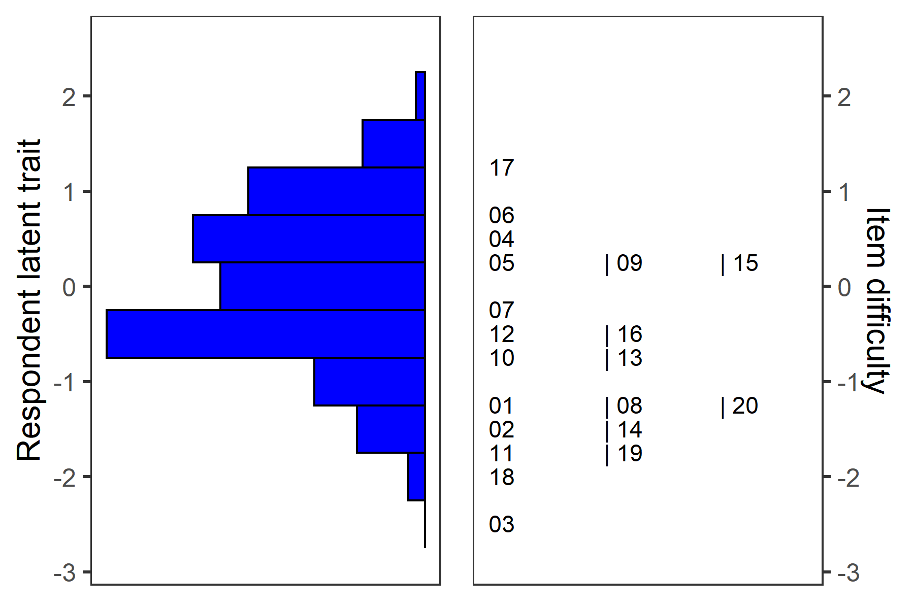
HCI dataset.
Item 17 was the most difficult; more than 1 SD above the mean ability was needed to answer this item correctly. Overall, the test is rather easy with most of the difficulty parameters lower than 0 (Figure 7.14).
The person-item map can be used when developing a test. If the test is used to distinguish respondents above a determined cut-score ability level, it would be desirable to add items with difficulty parameters around that value.
7.4.5 The lme4 and nlme packages
Both the lme4 and the nlme are general-purpose statistical packages used for the estimation of parameters in mixed-effect models, which implement the MML. We demonstrate here how the Rasch model may be fitted as a standard mixed-effect model using the glmer() function of the lme4 package.
In the example below, we use the HCIlong dataset. We fit the mixed effect model Equation 7.1 using -1 in the formula to remove the intercept and obtain estimated parameters for all items. Note that the variable item needs to be a factor. Resulting difficulty estimates are within the intercept-slope parametrization, explaining the difference in the sign.
library(lme4)
fit_rasch_lme4 <- glmer(rating ~ -1 + item + (1 | id), data = HCIlong,
                        family = binomial)
coef(fit_rasch_lme4)$id[1, -1]
##    Item1 Item2 Item3   Item4   Item5  Item6  Item7  Item8   Item9
## 1 0.9494 1.266 1.925 -0.4515 -0.2701 -0.653 0.2068 0.9911 -0.3128
## ...
While the computational time was considerably higher than with the mirt or ltm packages, the parameter estimates are similar. The package is limited to Rasch-type models, but it further allows for fitting a wide class of exploratory IRT models (De Boeck et al., 2011; see De Boeck & Wilson, 2004), including covariates, such as characteristics of respondents or items.
7.4.6 Bayesian IRT with the brms package
Bayesian estimation of IRT models can be done in R with the brms package, which provides a flexible interface to fit Bayesian models using Stan, which was previously introduced in Section 4.3.3.4. As an advantage, the same syntax used in the lmer() function can be used with the brm() function of the brms package. For our demonstration, we choose normal distribution with zero mean and SD of 3 as the prior distribution, both for the person and item parameters of the HCIlong dataset.
formula_1PL <- bf(rating ~ 1 + (1 | item) + (1 | id))
prior_1PL <- prior("normal(0, 3)", class = "sd", group = "id") +
             prior("normal(0, 3)", class = "sd", group = "item")

fit_1PL_brms <- brm(formula = formula_1PL, data = HCIlong, prior = prior_1PL,
                    family = brmsfamily("bernoulli", "logit"), seed = 123)
coef(fit_1PL_brms)$item[, , "Intercept"]
##    Estimate Est.Error     Q2.5    Q97.5
##  1    0.9602   0.09574  0.76907  1.15350
##  2    1.2570   0.09977  1.06261  1.45843
##  3    1.9112   0.11642  1.68002  2.14513
## ...
## 20    1.0797   0.09478  0.89838  1.26513
Once again, the estimation takes much longer than with the mirt or ltm packages, but similar parameter estimates are obtained for the Rasch model. The main advantage of the package and the Bayesian framework is its high flexibility in terms of model possibilities and extensions.
To summarize our practical demonstrations so far, the presented packages for estimation of the IRT models use, to some extent, different estimating methods. However, when the simplest Rasch model is used, and the parametrization is kept the same, they provide similar item parameter and person ability estimates (see the code in the Supplementary code for additional demonstrations).
7.5 Relationship between IRT and factor analysis
So far, we have conceptualized the IRT models as GLMMs, or nonlinear mixed-effect models. However, the IRT models can be formulated within other frameworks as well. Here we demonstrate how the IRT models are related to factor analysis (Bartholomew et al., 2011) discussed in Section 9.6.3.
In the two-parameter normal-ogive IRT model Equation 7.4 under the intercept-slope parametrization \[ \Pr(Y_{pi} = 1| \theta_p) = \Phi(\beta_{0i} + \beta_{1i}\theta_p), \] the intercept \(\beta_{0i}\) and the slope (item discrimination) \(\beta_{1i}\) are related to an item factor loading \(\alpha_i\) from the factor analysis model Equation 3.7 on the tetrachoric correlation matrix, and to a normal threshold \(\tau_i\) Equation 3.3 as follows:
\[ \beta_{0i} = \frac{- \tau_i}{\sqrt{1 - \alpha^2_i}}, \quad \quad \quad \beta_{1i} = \frac{\alpha_i}{\sqrt{1 - \alpha^2_i}}, \tag{7.19}\]
see Takane & De Leeuw (1987) and Kamata & Bauer (2008) for formal proof and more details.
Thus, if the slope and intercept parameters of the two-parameter normal-ogive IRT model Equation 7.4 are available, the factor loadings can be extracted as \[ \alpha_i = \frac{\beta_{1i}}{\sqrt{1 + \beta_{1i}^2}}, \quad \quad \quad \tau_i = \frac{- \beta_{0i}}{\sqrt{1 + \beta_{1i}^2}}. \] If, instead of the normal-ogive (probit-link) model, the 2PL (logit-link) IRT model Equation 7.3 is considered, in the intercept-slope parametrization Equation 7.7 approximate relationships hold for parameters \(D \beta_{1i}\) and \(D \beta_{0i}\), where \(D = 1.702\) is the scaling parameter used to align the logistic and the normal-ogive IRT model, as we discussed in Section 7.2.2.3 (also see Figure 7.3).
Relationship between IRT and factor analysis in R. We now demonstrate the relationship between parameter estimates in the IRT and factor analysis models with the HCI dataset. We first compute the tetrachoric correlation and extract the thresholds \(\tau_i\) using the tetrachoric() function of the psych package.
library(psych)
corHCI <- tetrachoric(HCI[, 1:20])$rho
(tau <- tetrachoric(HCI[, 1:20])$tau)
##  Item 1  Item 2  Item 3  Item 4  Item 5  Item 6  ...
## -0.5213 -0.6830 -1.0276  0.2430  0.1449  0.3517  ...
We then fit the one factor model Equation 3.7 using the fa() function of the psych package, as we did in Section 3.4.1, and we extract the factor loadings \(\alpha_i\).
FA1 <- fa(HCI[, 1:20], nfactors = 1, fm = "mle", cor = "poly")
(alpha <- c(FA1$loadings))
## [1] 0.4441 0.3863 0.6148 0.1987 0.4161 0.5133 ...
We now calculate the estimates of slope (item discrimination) \(\beta_{1i}\) and intercept \(\beta_{0i}\) according to Equation 7.19, while also multiplying the estimates by scaling parameter \(D = 1.702\). The denominator in Equation 7.19 is extracted as the estimated uniqueness in the factor analysis model.
q <- sqrt(c(FA1$uniquenesses)) # q = sqrt(1 - alpha^2)
D <- 1.702
beta1FA <- D * alpha / q # slope
beta0FA <- -D * tau / q  # intercept
Similar parameter estimates should be obtained from the IRT model. We use the 2PL IRT model Equation 7.3 fitted in Section 7.4.1 with the mirt() function of the mirt package. The item parameters are extracted this time in the default intercept-slope parametrization Equation 7.7.
beta1IRT <- coef(fit_2PL_mirt, simplify = TRUE)$items[,"a1"]
beta0IRT <- coef(fit_2PL_mirt, simplify = TRUE)$items[,"d"]
We can now print the set of parameters calculated from the IRT model and their counterparts estimated under the factor analytic model next to each other, and estimate the correlations between them.
rbind(beta1FA, beta1IRT)
##          Item 1 Item 2 Item 3 Item 4 Item 5 Item 6 Item 7 ...
## beta1FA  0.8437 0.7128 1.3269 0.3450 0.7788 1.0180 0.2621 ...
## beta1IRT 0.8509 0.7167 1.5745 0.3467 0.7275 1.0115 0.2257 ...
rbind(beta0FA, beta0IRT)
##          Item 1 Item 2 Item 3  Item 4  Item 5  Item 6 Item 7 ...
## beta0FA  0.9903 1.2602 2.2176 -0.4220 -0.2712 -0.6976 0.2027 ...
## beta0IRT 0.9754 1.2348 2.4033 -0.3995 -0.2545 -0.6761 0.1905 ...

cor(beta1FA, beta1IRT)
## [1] 0.9908
cor(beta0FA, beta0IRT)
## [1] 0.9987
The parameter estimates are very similar, and correlation between the estimates from the two frameworks is over \(0.99\).
Vice-versa, the mirt() function provides the estimated factor loadings F1 and item communalities h2 recalculated from the estimated parameters of the IRT model in the summary() output
summary(fit_2PL_mirt)
##             F1      h2
## Item 1  0.4472 0.19997
## Item 2  0.3881 0.15060 ...
which are similar to those obtained from the fa() function.
unclass(FA1$loadings)
##            ML1
## Item 1  0.4441
## Item 2  0.3863 ...

FA1$communalities
##  Item 1  Item 2  Item 3  Item 4  Item 5  Item 6  Item 7  Item 8  ...
##  0.1973  0.1492  0.3780  0.0395  0.1731  0.2635  0.0232  0.2804  ...
This concludes our empirical demonstration of the equivalence between the IRT and factor analysis models. So far, we have only considered the EFA models. However, the factor analysis framework will allow us also to build CFA models discussed in Section 3.4.6, as we will demonstrate in Chapter 8. We will also be able to include grouping variables and other covariates, which is typical for SEM, as we will discuss in Chapter 10.
7.6 IRT models in interactive application
Section IRT models of the ShinyItemAnalysis application allow fitting the dichotomous 1–4PL IRT models.
For each model, the IRT parametrization or the classical intercept-slope parametrization is offered, and the ICCs, IICs, and TIC are also provided. A table summarizing estimated item parameters is complemented with item fit statistics (Ames & Penfield, 2015). A table with estimated respondent abilities is offered for download, and the relationship between standardized total scores and estimated latent abilities (factor scores) is displayed in a scatter plot. A person-item (Wright) map is displayed for the Rasch and 1PL models. A model comparison tab offers comparison of model fit for the 1–4PL models using the AIC and BIC including their modifications. While the fitting of IRT models is mainly implemented by the mirt package, a sample R code is also provided for work in other packages.
In the interactive training section, the user can specify parameters \(a\), \(b\), \(c\), and \(d\) in the 4PL IRT model for two toy items. The latent ability \(\theta\) of a respondent can also be selected. The ICCs are then provided interactively displaying the probability of a correct answer for any \(\theta\) and highlighting this probability for selected \(\theta\). The IICs are also displayed comparing the two items by the amount of information they provide about a respondent’s given ability level.
A training section also contains interactive exercises where users may check their understanding of the IRT models. Interactive exercises include tasks involving sketching of the ICCs and IICs within given parameters and questions on the probabilities of correct answers and on the information provided by these items for respondents with certain ability levels.
7.7 Summary
In this chapter, we have introduced the IRT models for binary data, and we have discussed the general concepts, assumptions, and estimation methods for this class of models. We have then described several R packages which may be used to fit binary IRT models and discussed the differences and similarities between these packages. The relationship between the 2PL IRT model and the factor analytic model was demonstrated.