References

1

T.M. Cover and J.A. Thomas, Elements of Information Theory (J. Wiley & Sons, New York, 1991).

2

I.P. Cornfeld, S.V. Fomin, Ya.G. Sinai, Ergodic Theory (Springer, New York, 1982).

3

K. Petersen, Ergodic Theory (Cambridge University Press, Cambridge, 1983).

4

Ya. G. Sinai, Introduction to Ergodic Theory (Princeton University Press, Princeton, 1976).

5

H.G. Schuster, Deterministic Chaos, An Introduction (Physik, Weinheim, 1988).

6

Ya.B. Pesin, Russian Math. Surveys 32 (1977) 55.

7

P. Grassberger and I. Procaccia, Phys. Rev. A 28 (1983) 2591.

8

A.M. Fraser, IEEE Transactions on Information Theory 35 (1989) 245.

9

G. Mayer-Kress, (ed.), Dimensions and Entropies in Chaotic Systems (Springer, Berlin, 1986).

10

N.B. Abraham, A.M. Albano, A. Passamante and P.E. Rapp, (eds.), Measures of Complexity and Chaos (Plenum Press, New York, 1989).

11

M. Palus, Physica D 93 (1996) 64.

12

T.-P. Chiang, Acta Scientiarum Naturalium Universitatis Pekinensis 1 (1987) 25.

13

S. Ihara, Information Theory for Continuous Systems, (World Scientific, Singapore, 1993).

14

V.V. Anh, K.E. Lunney, Mathl. Comput. Modelling 21(9) (1995) 67.

15

J. Theiler, S. Eubank, A. Longtin, B. Galdrikian and J.D. Farmer, Physica D 58 (1992) 77.

16

M. Palus, Physica D 80 (1995) 186.

17

D.E. Sigeti, Physica D 82 (1995) 135.

18

S. Grossmann, S. Thomae, Z. Naturforsch. 32a (1977) 1353.

19

H. Mori, B.-C. So, T. Ose, Prog. Theor. Phys. 66 (1981) 4.

20

J.M. Lipton, K.P. Dabke, Phys. Lett. A 210 (1996) 290.

21

E.N. Lorenz, J. Atmos. Sci. 20 (1963) 130.

22

W.H. Press, B.P. Flannery, S.A. Teukolsky and W.T. Vetterling, Numerical recipes: The Art of Scientific Computing, (Cambridge Univ. Press, Cambridge, 1986).

23

H.G.E. Hentschel and I. Procaccia, Physica D 8 (1983) 435.

24

J.D. Farmer, E. Ott and J.A. Yorke, Physica D 7 (1983) 153.

25

The code is available at URL: http://www.users.interport.net/~ wolf/

26

A. Wolf, J.B. Swift, H.L. Swinney and J.A. Vastano, Physica D 16 (1985) 285.

27

R.C. Hilborn, Chaos and Nonlinear Dynamics: An Introduction for Scientists and Engineers. (Oxford University Press, New York, 1994).

  
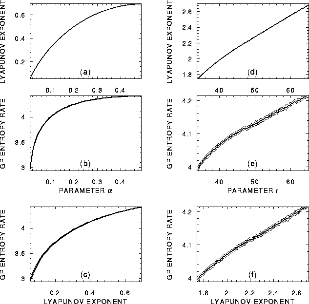
Figure 1: (a-c) Results for the baker map: a) The Lyapunov exponent as the analytic function of the parameter . b) The GP entropy rates estimated from 15 realizations of 16k time series (mean - thick line, mean SD - thin lines, coinciding with the mean) for different values of the parameter varying from 0.01 to 0.49 by step 0.005. c) Plot of GPER (the same line codes as in b) vs. LE. (d-f) Results for the Lorenz system: d) The positive Lyapunov exponents computed from the Lorenz equations for the parameter r varying from 33.75 to 65 by step 0.25. e) The GP entropy rates estimated from 15 realizations of 16k time series (mean - thick line, mean SD - thin lines) for different values of the parameter r varying as in plot d. f) Plot of GPER (the same line codes as before) vs. LE.

  
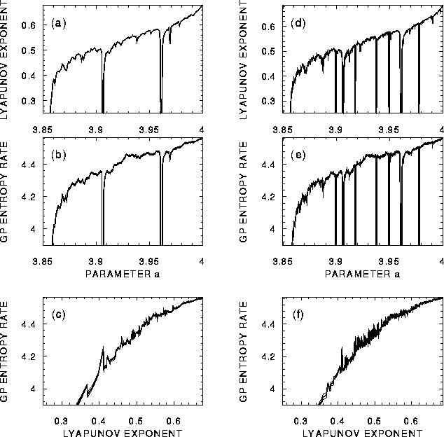
Figure 2: Results for the logistic map: a) The Lyapunov exponents computed from the map for the parameter a varying from 3.857 to 4 by step 0.001. b) The GP entropy rates estimated from 15 realizations of 16k time series (mean - thick line, mean SD - thin lines, coinciding with the mean) for different values of the parameter a varying as in plot a. c) Plot of GPER (the same line codes as before) vs. LE. Plots d, e, f: The same as the plots a, b, c, respectively, except of the parameter a varying by step 0.0003.

  
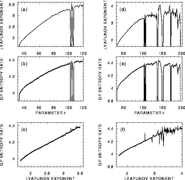
Figure 3: Further results for the Lorenz system: a) The positive Lyapunov exponents computed from the Lorenz equations for the parameter r varying from 33 to 120 by step 1. b) The GP entropy rates estimated from 15 realizations of 16k time series (mean - thick line, mean SD - thin lines, coinciding with the mean) for different values of the parameter r varying as in plot a. c) Plot of GPER (the same line codes as before) vs. LE. Plots d, e, f: The same as the plots a, b, c, respectively, except of the parameter r varying from 33 to 200 by step 1.

  
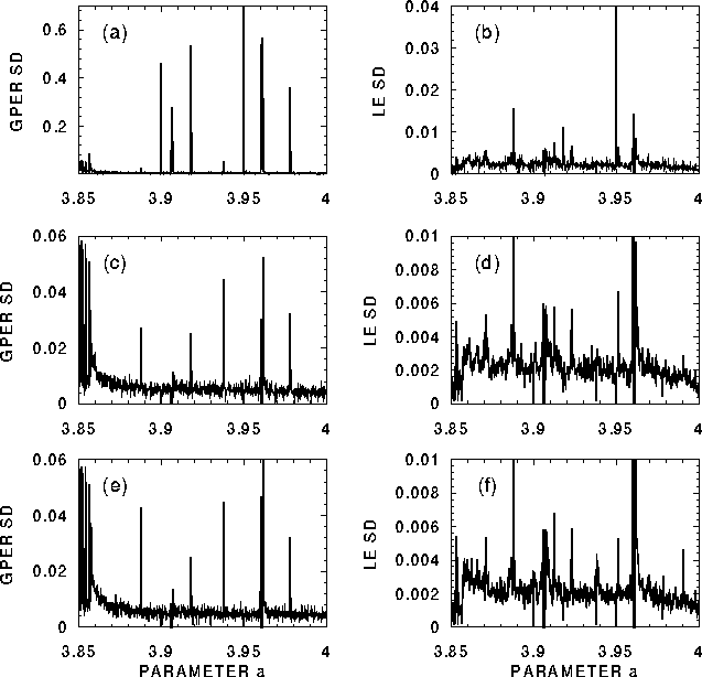
Figure: Standard deviation (square root of variance) of the GPER (a,c,e) and LE (b,d,f) estimates computed from the series generated by the logistic map after skipping zero (a,b), hundred thousand (c,d) and one billion (e,f) initial iterations to avoid influence of transients; plotted as the functions of the parameter a changing in the same range as in Fig. 2d-f.

  
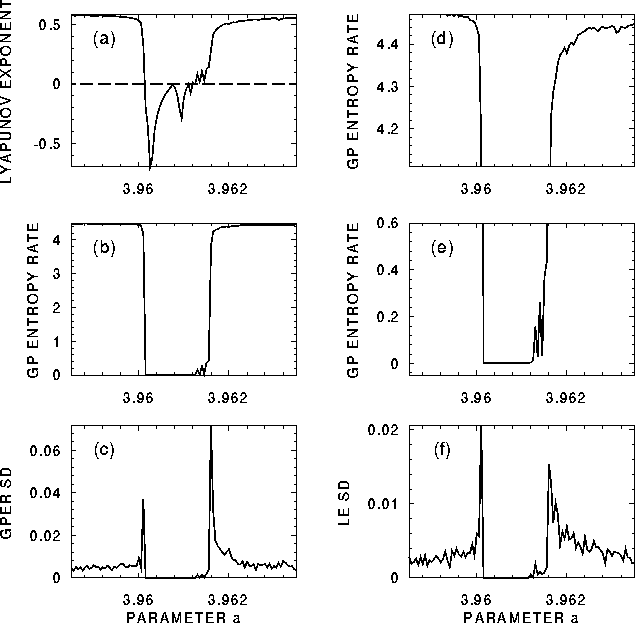
Figure 5: Detailed illustration of one of the bifurcations of the logistic map. Lyapunov exponent (a), GP entropy rate (b,d,e), standard deviation of the GPER estimate (c) and standard deviation of the LE estimate (f); plotted as functions of the parameter a. Upper and lower parts of the plot b are zoomed in the plots d and e, respectively.