Preparing source files
In your working directory,
So the structure should look as follows:
work_dir
+---celeba_crop_5k
¦ +--- 000001_crop.jpg
¦ +--- 000002_crop.jpg
¦ ¦
¦ +--- 006496_crop.jpg
¦
+---dcgan3X.py
+---fid_score.py
+---inception.py
+---list_attr_celeba.txt
Introduction
The purpose of this lab is to program a standard DCGAN [1]. You will work with a precoded DCGAN script that contains 4 tasks. The tasks are to program the appropriate functions so that the script works as whole and generates fake images. DCGAN learns on 5000 images from the well-known CelebA face photo dataset [2]. The structure of the script is standard for GAN learning. It consists of the following blocks:
[1] - https://arxiv.org/abs/1511.06434
[2] - https://mmlab.ie.cuhk.edu.hk/projects/CelebA.html
Submission
During lab we go through the script and you will gradually work on the tasks. Each task has attached its testing function to let you know if corresponding code works properly. If it is so, solving the task is awarded by points. They sums to 100 points.
To evaluate your HW, send a script for automatic evaluation (AE). It must be named dcgan3X.py. AE will run the same test functions you already have in the script. You must score 80 or more points for the HW to pass.
Data pipeline
A data pipeline ensures
flow of learning data. We use the standard PyTorch template given by a combination
of PyTorch Dataset and DataLoader classes [1]. We customize the Dataset class
for our needs - class CustomImageDataset.
CustomImageDataset class must contain the __len__ and __getitem__ methods in
addtion to the standard initialization __init__ method.
The first one specifies the number of items in the db (5000 in our case) and __getitem__ returns the corresponding image based on the input index. Images in celeba_crop_5k directory are in 128x128 resolution. In the preprocessing part of the __getitem__ method we reshape them to 64x64 resolution to make the network's processing computationally easier. We use the pillow library whose ToPILimage method returns the image as a tensor after reading it from the file. The images are in the standard RBG format so the corresponding tensor is 3 x 64 x 64 in the range of integer values 0 to 255.
In the preprocessing part
we need rescaling to float32 values in the range [-1, 1].
This is the first (and very easy) task to add the appropriate scale&shift
one-line code.
# ---
TASK 1 - rescale the image tensor from range 0..255 to range [-1, 1] (10 points)
#---
[1] - https://pytorch.org/tutorials/beginner/basics/data_tutorial.html
Generator
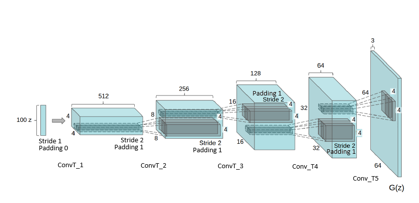
Generator is one of the two neural networks that combine into a GAN. In DCGAN, the generator is realized by means of transposed convolutional operations. Generated 64 x 64 images are represented by a tensor of three (RBG) channels, i.e. as tensors of dimension 3 x 64 x 64. They are generated by gradually processing random noise of low dimension (in our case it is 100). The generated image is created sequentially in single blocks, which consist of transposed convolutions (ConvTransposed2d [1]) that are responsible for increase in the spatial dimension; then regularization is performed by batch-normalization (BatchNorm) and finally non-linearity is added using the ReLU layer. Change of the spatial dimension going over particular blocks goes as follows:
(noise) 100x1x1 -> 512x4x4 -> 256x8x8 -> 128x16x16 -> 64x32x32 -> 3x64x64 (output)
Output is further modified using Tanh function to be assured that it is in range [-1,1]. When obtaining final image it must be rescaled back (inverse operation to preprocessing) to integer 0..255 scale.
The dimension upscaling is performed by ConvTransposed2d convolutions. PyTorch call of ConvTransposed layer writes as:
nn.ConvTranspose2d(in_channels, out_channels, kernel_size, stride, padding, ... , dilation=1, output_padding=0)
If the dimension of a square tensor (image) is D_in, i.e., it is in_channels x D_in x D_in tensor, then the ouput tensor's dimensions are out_channels x D_out x D_out, where
D_out=(D_in-1)*stride-2*padding+dilation*(kernel_size-1)+output_padding+1
Examples of this computation are:
OBSERVATION: Let kernel=4,
stride=2 and padding=1 as in the 2nd example
above and D_in is arbitrary.
Then the D_out formula writes as
D_out=(D_in-1)*2-2*1+1*(4-1)+0+1 = (D_in-1)*2+3+1=2*D_in-2-2+4 = 2*D_in
Hence the selected combination of parameters doubles the input dimension irrespective of its concrete value.
# ---
TASK 2 - is to specify generator's layers so that dimension upscaling follows
the prescribed patern - see the script for template (35 pts.)
#----
[1] - https://pytorch.org/docs/stable/generated/torch.nn.ConvTranspose2d.html
[*] - https://github.com/vdumoulin/conv_arithmetic/blob/master/README.md
- visualisations
Discriminator
Output of the discriminator is the probability that the input image is real. Hence the output is a real number from the unit interval [0,1]. Where 0 corresponds to a fake image and 1 to certainly a real image. The discriminator is implemented as a classical convolutional structure, where within each block the input dimension of the 3 x 64 x 64 image is reduced by convolution down to the output probability realized by the last sigmoidal layer. In each block, a batch normalization (BatchNorm) is used as the regularization layer and a Leaky ReLU as the nonlinearity. The change of the spatial dimension goes as follows:
(input) 3x64x64 ->64x32x32 -> 128x16x16 -> 256x8x8 -> 512x4x4 -> 1x1x1 -> scalar (output)
Dimension upscaling is done using the Conv2d convolutions [1]. PyTorch call of Conv2d layer writes as:
nn.Conv2d(in_channels, out_channels, kernel_size, stride, padding, ... , dilation=1)
If the input dimension of image is D_in, i.e., it is in_channels x D_in x D_in tensor, then ouput tensor is out_channels x D_out x D_out, with
D_out=[(D_in+2*padding-dilation*(kernel_size-1)-1)/stride + 1]_+
where [.]_+ denotes the lower integer part.
Examples of this computation are:
# ---
TASK 3- is to specify discriminator's layers so that dimension downscaling follows
the prescribed patern - see the script for template (35 pts.)
#----
[1] - https://pytorch.org/docs/stable/generated/torch.nn.Conv2d.html
Losses
Following the theorethical derivation in [1], parameters of discriminator (D) and generator (G) are optimized to reach the saddle point of the functional (1). This is done in alternating manner when parameters of D are optimized for G fixed (the discriminator loss) and in the second step the parameters of G are optimized for D fixed (the generator loss).

In practice, expected values are replaced by their sample counter parts when real images are used in the first term and fake images in the second term (corresponding to the output of generator G(z)).
As optimizers in PyTorch are used in minimizing mode. The discriminator loss
is reverted to its negative counterpart and then minimized instead of original
maximization. This gives this PyTorch specification of the discriminator loss:
disc_loss = -torch.mean(torch.log(disc_real) + torch.log(1. - disc_fake))
In the case of generator loss, only optimization of the second term applies
as G is not present in the first one. Paper [1] advises instead of minimizing
E_z[log(1-G(z))] to maximize log(G(z)) to get stronger gradients:
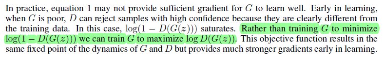
This advice is used in our script. Again, reverting maximization to minimization applies in the specification of the generator loss as E_z[-log(G(z))].
# ---
TASK 4 is to specify generator loss in function gen_loss similarly as it is
done in function disc_loss for the discriminator (20 pts.)
#---
Optimizers
Both discriminator and generator
use their own optimizers. They are the standard Adam optimizers with
learning rate set to lr=0.0002 and beta1 = 0.5, beta2 =0.999 parameters.
They differ in what parameters
they optimize. The first applies to the discriminator.parameters() and the second
to the generator.parameters().
Training loop
The training loop follows Algorithm 1 listing from [1], with the exception of using the adjusted version of generator loss as explained above.
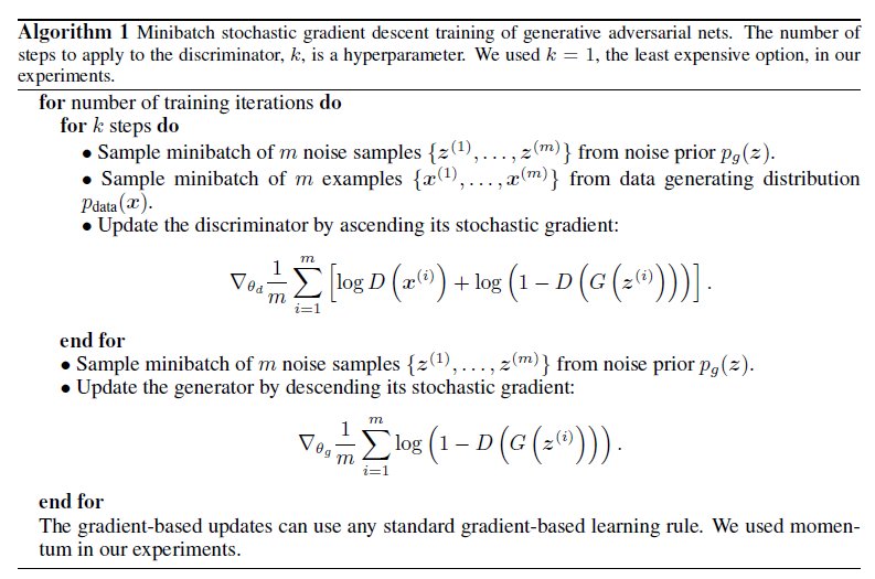
We specify number of epochs of learning. Real images are delivered using the specified DataLoader connected to the celeba_crop_5k directory containing real images. Further, optimization of discriminator is practically done with the following code:
For the discriminator
and similarly for the generator:
Output
The script creates the results_5k subdirectory where generated fake images are stored using the shb2 helper function. This is done at the very beginning when real images are reported, then fake images are saved until epoch=10 and further each 10-th epoch. The images are arranged on 4x4 canvas so 16 images are saved during each record.
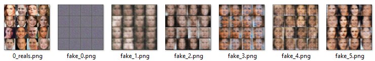
FID score computation
We start with computation of FID (Frechet Inception Distance) between two chunks of real images to obtain a lower bound on the FID (the size of the chunks is controlled by the FID_BATCH parameter). This involves calculating mu_1, sgm_1 and mu_2, sgm_2 for each chunk. The first chunk parameters are then used to calculate FID for the generated images during training. The script reports FID for the generated images every 10-th epoch and the sequence should decrease towards the lower bound as the quality of the generated images improves, which could be visually checked in the results_5k subdirectory.
[1] Generative Adversial
Networks - https://arxiv.org/abs/1406.2661
[2] FID - Coursera
[3] InceptionV3 - Coursera